洛伦兹吸引力
这是使用mplot3d在3维空间中绘制Edward Lorenz 1963年的“确定性非周期流”的示例。
注意:因为这是一个简单的非线性ODE,使用SciPy的ode求解器会更容易完成,但这种方法仅取决于NumPy。
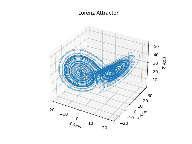
import numpy as npimport matplotlib.pyplot as plt# This import registers the 3D projection, but is otherwise unused.from mpl_toolkits.mplot3d import Axes3D # noqa: F401 unused importdef lorenz(x, y, z, s=10, r=28, b=2.667):'''Given:x, y, z: a point of interest in three dimensional spaces, r, b: parameters defining the lorenz attractorReturns:x_dot, y_dot, z_dot: values of the lorenz attractor's partialderivatives at the point x, y, z'''x_dot = s*(y - x)y_dot = r*x - y - x*zz_dot = x*y - b*zreturn x_dot, y_dot, z_dotdt = 0.01num_steps = 10000# Need one more for the initial valuesxs = np.empty((num_steps + 1,))ys = np.empty((num_steps + 1,))zs = np.empty((num_steps + 1,))# Set initial valuesxs[0], ys[0], zs[0] = (0., 1., 1.05)# Step through "time", calculating the partial derivatives at the current point# and using them to estimate the next pointfor i in range(num_steps):x_dot, y_dot, z_dot = lorenz(xs[i], ys[i], zs[i])xs[i + 1] = xs[i] + (x_dot * dt)ys[i + 1] = ys[i] + (y_dot * dt)zs[i + 1] = zs[i] + (z_dot * dt)# Plotfig = plt.figure()ax = fig.gca(projection='3d')ax.plot(xs, ys, zs, lw=0.5)ax.set_xlabel("X Axis")ax.set_ylabel("Y Axis")ax.set_zlabel("Z Axis")ax.set_title("Lorenz Attractor")plt.show()
下载这个示例

若有收获,就点个赞吧
0 人点赞
