1.数学原理

1801年，意大利天文学家朱赛普·皮亚齐发现了第一颗小行星谷神星。经过40天的跟踪观测后，由于谷神星运行至太阳背后，使得皮亚齐失去了谷神星的位置。随后全世界的科学家利用皮亚齐的观测数据开始寻找谷神星，但是根据大多数人计算的结果来寻找谷神星都没有结果。只有时年24岁的高斯所计算的谷神星的轨道，被奥地利天文学家海因里希·奥尔伯斯的观测所证实，使天文界从此可以预测到谷神星的精确位置。同样的方法也产生了哈雷彗星等很多天文学成果。高斯使用的方法就是最小二乘法，该方法发表于1809年他的著作《天体运动论》中 。其实法国科学家勒让德于1806年独立发明“最小二乘法”，但因不为世人所知而默默无闻 。

这里涉及到的数学原理是“最小二乘法”，更底层的数学基础是 偏导数；
大陆地区翻译成“最小二乘法”，台湾地区翻译成“最小平方法”。

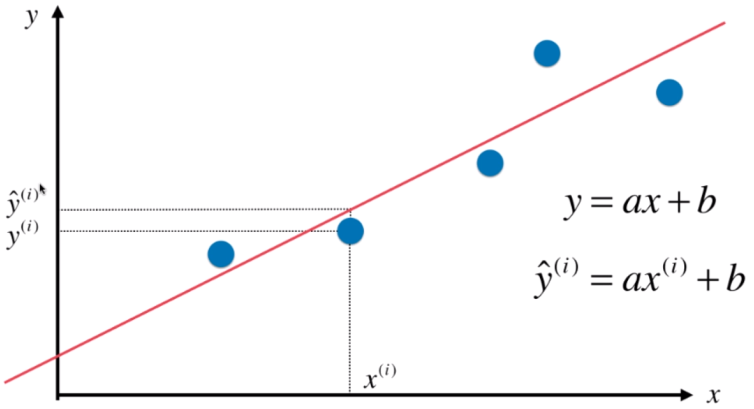
• 预测值拟合直线为：
• 实际值为 :

为了让拟合直线和贴合数据，希望 的值尽量小，但是可能是负值， 因此可以表示两者的差距，但是为了方便计算采用平方的形式： ，因为后面要用偏导数计算。

• 目标：使尽可能小。即找到a和b，使得尽可能小。

也叫损失函数(loss function)。
某类机器学习的思路：通过最优化损失函数或者效用函数，获得机器学习模型。

• 参数表达式

导数为0的地方，就是极值的地方。（分别对a ，b求偏导为0时，可得：）
，

2.编码实现

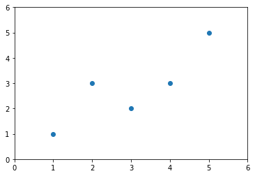
准备数据

import numpy as np
import matplotlib.pyplot as plt
x = np.array([1., 2., 3., 4., 5.])
y = np.array([1., 3., 2., 3., 5.])
plt.scatter(x, y)
plt.axis([0, 6, 0, 6])
plt.show()

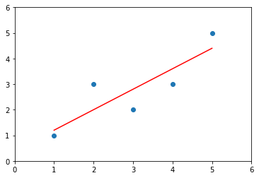
建模

# 求x,y的均值
x_mean = np.mean(x)
y_mean = np.mean(y)
# 求系数a,b
num = 0.0
d = 0.0
for x_i, y_i in zip(x, y):
    num += (x_i - x_mean) * (y_i - y_mean)
    d += (x_i - x_mean) ** 2
a = num/d
b = y_mean - a * x_mean    
y_hat = a * x + b
plt.scatter(x, y)
plt.plot(x, y_hat, color='r')
plt.axis([0, 6, 0, 6])
plt.show()

预测

x_predict = 6
y_predict = a * x_predict + b
print(y_predict)  # 5.2

3.模型封装

class SimpleLinearRegression1:
    def __init__(self):
        """初始化Simple Linear Regression 模型"""
        self.a_ = None
        self.b_ = None
    def fit(self, x_train, y_train):
        """根据训练数据集x_train,y_train训练Simple Linear Regression模型"""
        assert x_train.ndim == 1, \
            "Simple Linear Regressor can only solve single feature training data."
        assert len(x_train) == len(y_train), \
            "the size of x_train must be equal to the size of y_train"
        x_mean = np.mean(x_train)
        y_mean = np.mean(y_train)
        num = 0.0  # num为表达式的分子
        d = 0.0  # d 为表达式的分母
        for x, y in zip(x_train, y_train):
            num += (x - x_mean) * (y - y_mean)
            d += (x - x_mean) ** 2
        self.a_ = num / d
        self.b_ = y_mean - self.a_ * x_mean
        return self
    def predict(self, x_predict):
        """给定待预测数据集x_predict，返回表示x_predict的结果向量"""
        assert x_predict.ndim == 1, \
            "Simple Linear Regressor can only solve single feature training data."
        assert self.a_ is not None and self.b_ is not None, \
            "must fit before predict!"
        return np.array([self._predict(x) for x in x_predict])
    def _predict(self, x_single):
        """给定单个待预测数据x，返回x的预测结果值"""
        return self.a_ * x_single + self.b_
    def __repr__(self):
        return "SimpleLinearRegression1()"

# 使用封装的模型
from playML.SimpleLinearRegression import SimpleLinearRegression1
x = np.array([1., 2., 3., 4., 5.])
y = np.array([1., 3., 2., 3., 5.])
reg1 = SimpleLinearRegression1()
reg1.fit(x, y)  # 建模：得到参数 reg1.a_ = 0.8 , reg1.b_ = 0.4
# 预测单个值
x_predict = 6
reg1.predict(np.array([x_predict]))  # array([5.2])
y_hat1 = reg1.predict(x)
# 预测多个值
y_hat1 = reg1.predict(x)  # array([1.2, 2. , 2.8, 3.6, 4.4])
# 可视化
plt.scatter(x, y)
plt.plot(x, y_hat1, color='r')
plt.axis([0, 6, 0, 6])
plt.show()

4.模型优化

提升性能：向量化代替for循环（计算机的算法优化）

class SimpleLinearRegression2:
    def __init__(self):
        """初始化Simple Linear Regression模型"""
        self.a_ = None
        self.b_ = None
    def fit(self, x_train, y_train):
        """根据训练数据集x_train,y_train训练Simple Linear Regression模型"""
        assert x_train.ndim == 1, \
            "Simple Linear Regressor can only solve single feature training data."
        assert len(x_train) == len(y_train), \
            "the size of x_train must be equal to the size of y_train"
        x_mean = np.mean(x_train)
        y_mean = np.mean(y_train)
        #  向量化代替for循环
        self.a_ = (x_train - x_mean).dot(y_train - y_mean) / (x_train - x_mean).dot(x_train - x_mean)
        self.b_ = y_mean - self.a_ * x_mean
        return self
    def predict(self, x_predict):
        """给定待预测数据集x_predict，返回表示x_predict的结果向量"""
        assert x_predict.ndim == 1, \
            "Simple Linear Regressor can only solve single feature training data."
        assert self.a_ is not None and self.b_ is not None, \
            "must fit before predict!"
        return np.array([self._predict(x) for x in x_predict])
    def _predict(self, x_single):
        """给定单个待预测数据x_single，返回x_single的预测结果值"""
        return self.a_ * x_single + self.b_
    def __repr__(self):
        return "SimpleLinearRegression2()"

from playML.SimpleLinearRegression import SimpleLinearRegression2
reg2 = SimpleLinearRegression2()
reg2.fit(x, y)  # 建模：得到参数 reg1.a_ = 0.8 , reg1.b_ = 0.4
# 预测多个值
y_hat2 = reg2.predict(x)
# 可视化
plt.scatter(x, y)
plt.plot(x, y_hat2, color='r')
plt.axis([0, 6, 0, 6])
plt.show()

5.性能测试

m = 1000000  # 百万级数据
big_x = np.random.random(size=m)
big_y = big_x * 2 + 3 + np.random.normal(size=m)
%timeit reg1.fit(big_x, big_y)  # 耗时1秒
# 1.02 s ± 26.9 ms per loop (mean ± std. dev. of 7 runs, 1 loop each)
%timeit reg2.fit(big_x, big_y)  # 耗时14毫秒
# 14.2 ms ± 91.4 µs per loop (mean ± std. dev. of 7 runs, 100 loops each)
reg1.a_  # 2.0001613808322065
reg1.b_  # 3.002296137768425
reg2.a_  # 2.000161380832136
reg2.b_  # 3.00229613776846

6.评价指标

常用指标

MSE、RMSE、MAE
同样一个线性回归任务，使尽可能小，就能评价算法的优劣吗？
显然不能，因为算法的数据规模不同，误差也因此可能不同，因此得到的模型也无法比较优劣。

MSE

Mean Squared Errod 均方误差

RMSE

Root Mean Squared Errod 均方根误差

优点：相比MSE的单位为平方，RMSE的单位和原数据保持一致。

MAE

Mean Absolute Errod 平均绝对误差

优点：相比MSE的单位为平方，MAE的单位和原数据保持一致。

编码实现

# model_selection.py
# 作用： 切分训练集和测试集
import numpy as np
def train_test_split(X, y, test_ratio=0.2, seed=None):
    """将数据 X 和 y 按照test_ratio分割成X_train, X_test, y_train, y_test"""
    assert X.shape[0] == y.shape[0], \
        "the size of X must be equal to the size of y"
    assert 0.0 <= test_ratio <= 1.0, \
        "test_ration must be valid"
    if seed:
        np.random.seed(seed)
    shuffled_indexes = np.random.permutation(len(X))
    test_size = int(len(X) * test_ratio)
    test_indexes = shuffled_indexes[:test_size]
    train_indexes = shuffled_indexes[test_size:]
    X_train = X[train_indexes]
    y_train = y[train_indexes]
    X_test = X[test_indexes]
    y_test = y[test_indexes]
    return X_train, X_test, y_train, y_test

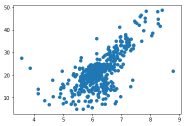
import numpy as np
import matplotlib.pyplot as plt
from sklearn import datasets
# 波士顿房产数据
boston = datasets.load_boston()
boston.keys()  # dict_keys(['data', 'target', 'feature_names', 'DESCR'])
# print(boston.DESCR)  # 查看数据集详情
boston.feature_names  # array(['CRIM', 'ZN', 'INDUS', 'CHAS', 'NOX', 'RM', 'AGE', 'DIS', 'RAD', 'TAX', 'PTRATIO', 'B', 'LSTAT'], dtype='<U7')
x = boston.data[:,5] # 只使用房间数量这个特征
x.shape  # (506,)
# 可视化
plt.scatter(x, y)
plt.show()

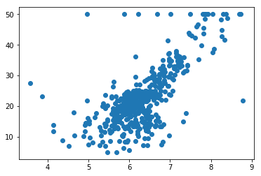
np.max(y)  # 50.0
x = x[y < 50.0]
y = y[y < 50.0]
x.shape  # (490,)
plt.scatter(x, y)
plt.show()

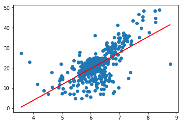
from playML.model_selection import train_test_split
# 切分数据集
x_train, x_test, y_train, y_test = train_test_split(x, y, seed=666)
x_train.shape  # (392,)
y_train.shape  # (392,)
x_test.shape  # (98,)
y_test.shape  # (98,)
# 建模
from playML.SimpleLinearRegression import SimpleLinearRegression
reg = SimpleLinearRegression()
reg.fit(x_train, y_train)
reg.a_  # 7.8608543562689555
reg.b_  # -27.459342806705543
# 可视化
plt.scatter(x_train, y_train)
plt.plot(x_train, reg.predict(x_train), color='r')
plt.show()

# MSE
mse_test = np.sum((y_predict - y_test)**2) / len(y_test)
mse_test  # 24.156602134387438

# RMSE
from math import sqrt
rmse_test = sqrt(mse_test)
rmse_test  # 4.914936635846635

# MAE
mae_test = np.sum(np.absolute(y_predict - y_test))/len(y_test)
mae_test  # 3.5430974409463873

封装评价指标

import numpy as np
from math import sqrt
def accuracy_score(y_true, y_predict):
    """计算y_true和y_predict之间的准确率"""
    assert len(y_true) == len(y_predict), \
        "the size of y_true must be equal to the size of y_predict"
    return np.sum(y_true == y_predict) / len(y_true)
def mean_squared_error(y_true, y_predict):
    """计算y_true和y_predict之间的MSE"""
    assert len(y_true) == len(y_predict), \
        "the size of y_true must be equal to the size of y_predict"
    return np.sum((y_true - y_predict)**2) / len(y_true)
def root_mean_squared_error(y_true, y_predict):
    """计算y_true和y_predict之间的RMSE"""
    return sqrt(mean_squared_error(y_true, y_predict))
def mean_absolute_error(y_true, y_predict):
    """计算y_true和y_predict之间的MAE"""
    return np.sum(np.absolute(y_true - y_predict)) / len(y_true)

from playML.metrics import mean_squared_error
from playML.metrics import root_mean_squared_error
from playML.metrics import mean_absolute_error
mean_squared_error(y_test, y_predict)  # 24.156602134387438
root_mean_squared_error(y_test, y_predict)  # 4.914936635846635
mean_absolute_error(y_test, y_predict)  # 3.5430974409463873

scikit-learn中的MSE和MAE

scikit-learn 中没有实现 RMSE。

from sklearn.metrics import mean_squared_error
from sklearn.metrics import mean_absolute_error
mean_squared_error(y_test, y_predict)  # 24.156602134387438
mean_absolute_error(y_test, y_predict)  # 3.5430974409463873

最好指标

R Squared

最好的衡量线性回归法的指标。

使用我们的模型预测产生的错误
基准模型：使用 预测产生的错误（不考虑x，预测值均为，误差肯定比上式大）

• R2越大越好。当我们的预测模型不犯任何错误是，R^2得到最大值1
• 当我们的模型等于基准模型时，R^2为0
• 如果R2<0，说明我们学习到的模型还不如基准模型。此时，很有可能我们的数据不存在任何线性关系。

封装R Score

# metrics.py
import numpy as np
from math import sqrt
def accuracy_score(y_true, y_predict):
    """计算y_true和y_predict之间的准确率"""
    assert len(y_true) == len(y_predict), \
        "the size of y_true must be equal to the size of y_predict"
    return np.sum(y_true == y_predict) / len(y_true)
def mean_squared_error(y_true, y_predict):
    """计算y_true和y_predict之间的MSE"""
    assert len(y_true) == len(y_predict), \
        "the size of y_true must be equal to the size of y_predict"
    return np.sum((y_true - y_predict)**2) / len(y_true)
def root_mean_squared_error(y_true, y_predict):
    """计算y_true和y_predict之间的RMSE"""
    return sqrt(mean_squared_error(y_true, y_predict))
def mean_absolute_error(y_true, y_predict):
    """计算y_true和y_predict之间的MAE"""
    assert len(y_true) == len(y_predict), \
        "the size of y_true must be equal to the size of y_predict"
    return np.sum(np.absolute(y_true - y_predict)) / len(y_true)
def r2_score(y_true, y_predict):
    """计算y_true和y_predict之间的R Square"""
    return 1 - mean_squared_error(y_true, y_predict)/np.var(y_true)

from playML.metrics import r2_score
r2_score(y_test, y_predict)  # 0.61293168039373225

scikit-learn中的 r2_score

scikit-learn中的LinearRegression中的score返回r2_score:http://scikit-learn.org/stable/modules/generated/sklearn.linear_model.LinearRegression.html

from sklearn.metrics import r2_score
r2_score(y_test, y_predict)  # 0.61293168039373236