准备数据

import numpy as np
import matplotlib.pyplot as plt
from sklearn.linear_model import LinearRegression
# 1. 数据展示：了解数据，可以是csv读取，也可以直接copy进来
years = np.arange(2009, 2020)
sales = np.array([0.52, 9.36, 33.6, 132, 352, 571, 912, 1207, 1682, 2135, 2684])
print(years)
print(sales)

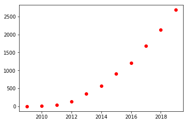
可视化

一般使用散点图

plt.scatter(years, sales, c='red')

初步判断

多项式回归(3阶)

y = a*x^3 + b*x^2 + c*x + d
1: 1 1 1
2: 8 4 2
3: 27 9 3

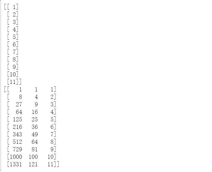
数据预处理

model_y = sales
model_x = (years - 2008).reshape(-1, 1)  # 任意行，一列
print(model_x)
model_x = np.concatenate([model_x ** 3, model_x ** 2, model_x], axis=1)
print(model_x)

建模

# 4. 创建回归模型（多项式->1元3次）
model = LinearRegression()
# 5. 数据训练
model.fit(model_x, model_y)
# 6. 获取系数、截距 -> 声明方程式
print('系数：', model.coef_)  # 系数： [  -0.20964258   34.42433566 -117.85390054]
print('截距：', model.intercept_)  # 截距： 90.12060606060629

y = -0.20964258*x^3 + 34.42433566*x^2 + -117.85390054*x + 90.12060606060629

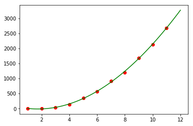
绘图

# 7. 添加趋势线：想象成画折线图，x:1~11,12 y:带入公式之后得到的
trend_x = np.linspace(1, 12, 100)
fun = lambda x: -0.20964258 * x ** 3 + 34.42433566 * x ** 2 + -117.85390054 * x + 90.12060606060629
trend_y = fun(trend_x)
# print(type(fun))
# print(trend_x)
# print(trend_y)
years_no = years - 2008
plt.scatter(years_no, sales, c='red')  # 画散点图
plt.plot(trend_x, trend_y, c='green')  # 画趋势线
plt.show()

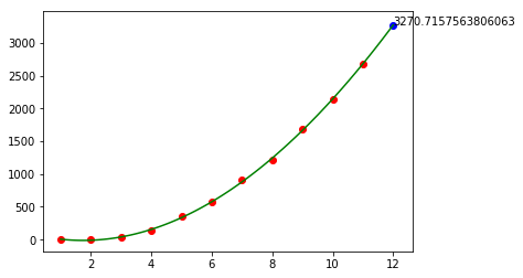
预测

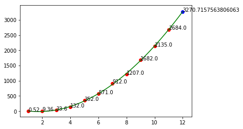
# 8. 预测2020年的销售额
print('2020年销售额预测：', fun(12))
years_no = years - 2008
plt.scatter(years_no, sales, c='red')
plt.scatter(12, fun(12), c='blue')
plt.plot(trend_x, trend_y, c='green')
# 加数据标签
plt.annotate(fun(12), xy=(12, fun(12)))  # annotate : (参数1：注释文本的内容, 参数2：被注释的坐标点)

给其它坐标加标签

for i in range(11):
    plt.annotate(sales[i], xy=(years_no[i], sales[i]))
plt.show()

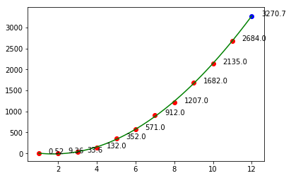
调整标签的位置

# x右移0.5，y下移0.5
plt.annotate(round(fun(12), 1), xy=(12, fun(12)), xytext=(12 + 0.5, fun(12) - 0.5))
for i in range(11):
    plt.annotate(sales[i], xy=(years_no[i], sales[i]), xytext=(years_no[i] + 0.5, sales[i] - 0.5))
plt.show()