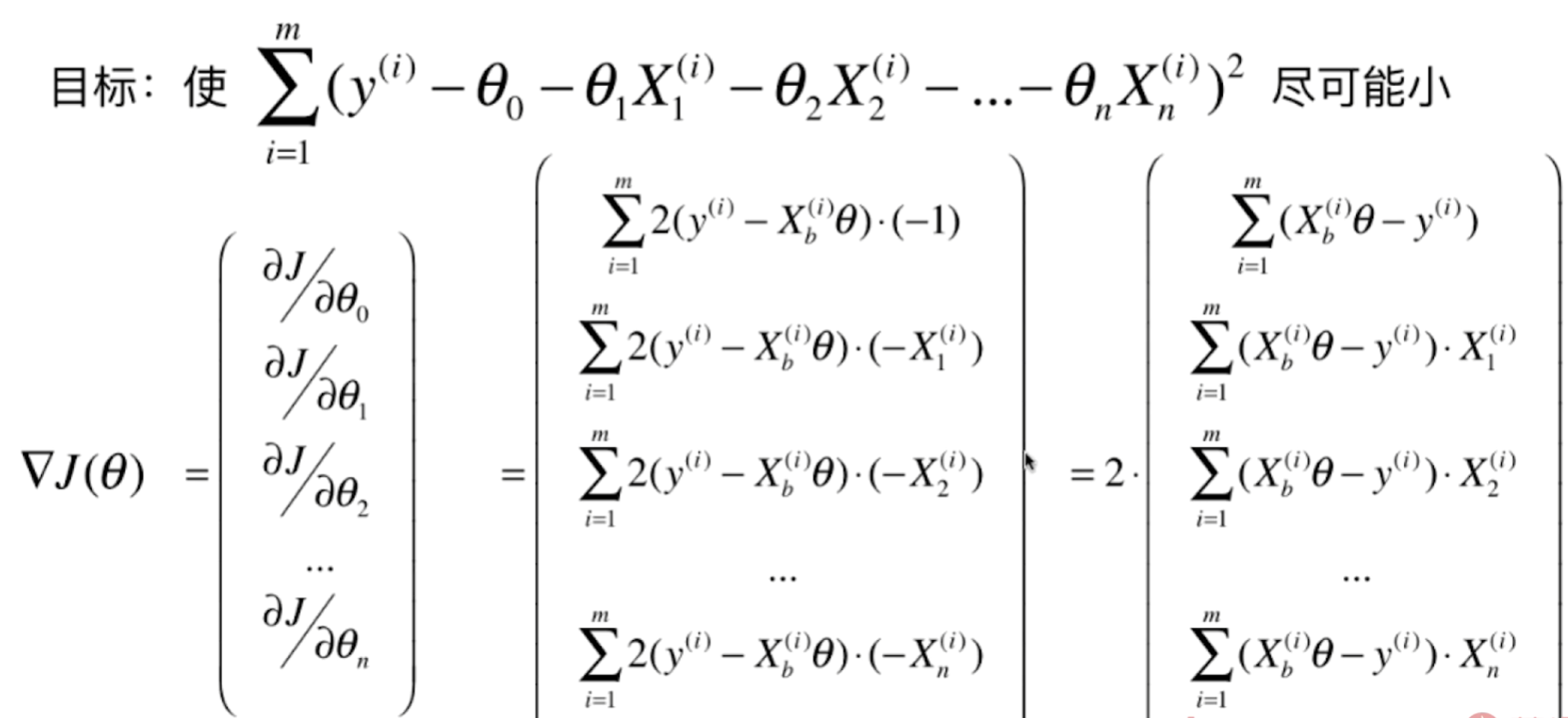
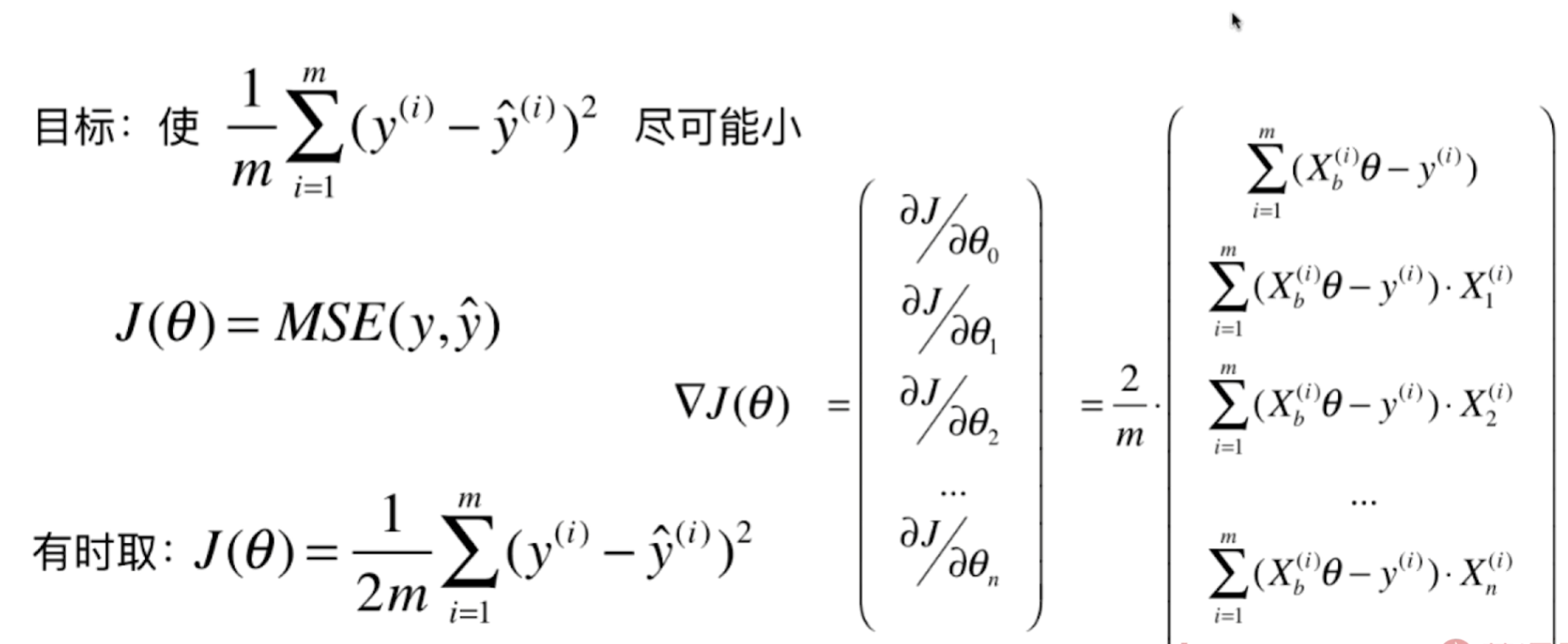
多元回归损失函数
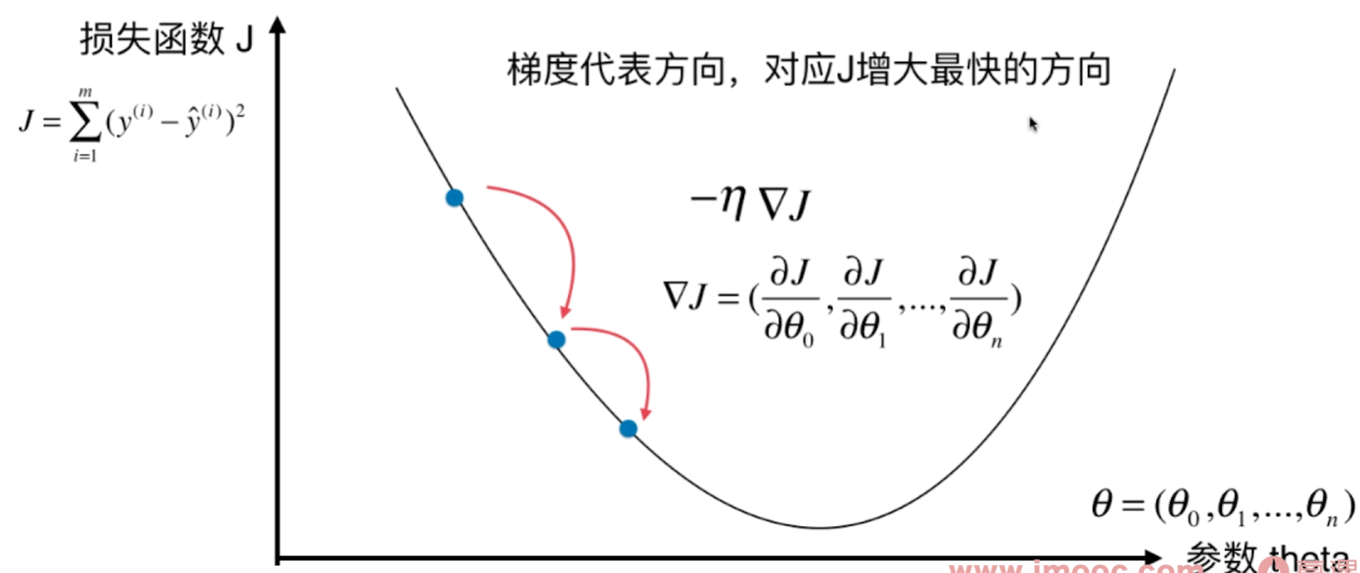
二元回归图解
损失函数公式推导
编码实现
准备数据
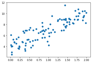
import numpy as npimport matplotlib.pyplot as pltnp.random.seed(666)x = 2 * np.random.random(size=100)y = x * 3. + 4. + np.random.normal(size=100)x
array([1.40087424, 1.68837329, 1.35302867, 1.45571611, 1.90291591,0.02540639, 0.8271754 , 0.09762559, 0.19985712, 1.01613261,0.40049508, 1.48830834, 0.38578401, 1.4016895 , 0.58645621,1.54895891, 0.01021768, 0.22571531, 0.22190734, 0.49533646,0.0464726 , 1.45464231, 0.68006988, 0.39500631, 1.81835919,1.95669397, 1.06560509, 0.5182637 , 1.16762524, 0.65138131,1.77779863, 1.25280905, 1.63774738, 1.09469084, 0.83342401,1.48609438, 0.73919276, 0.15033309, 1.55038596, 0.43881849,0.15868425, 0.97356104, 0.3073478 , 1.65693027, 0.38273714,0.54081791, 1.12206884, 1.80476078, 1.70357668, 0.83616392,0.78695254, 0.03244103, 0.59842674, 0.70755644, 1.78700533,1.57227314, 1.54277385, 0.84010971, 1.55205028, 0.92861629,0.36354033, 1.76805121, 1.43758454, 1.3437626 , 0.51312727,0.86160364, 0.03290715, 0.46998765, 1.02234262, 0.58401848,1.00378702, 0.99654626, 0.20754305, 0.89288623, 1.93837834,1.47694224, 1.43910122, 1.78608677, 1.92534936, 0.39410046,1.42917993, 0.32384788, 1.73250954, 1.24764049, 1.91891025,1.04828408, 0.07286576, 1.45374316, 0.00781969, 0.100588 ,1.98398463, 0.424515 , 1.89474133, 0.9030811 , 1.99758935,1.29500298, 1.40448142, 0.85916353, 0.33554952, 0.23626619])
X = x.reshape(-1, 1) # 转二维,方便处理多维数据X[:20]
array([[1.40087424],[1.68837329],[1.35302867],[1.45571611],[1.90291591],[0.02540639],[0.8271754 ],[0.09762559],[0.19985712],[1.01613261],[0.40049508],[1.48830834],[0.38578401],[1.4016895 ],[0.58645621],[1.54895891],[0.01021768],[0.22571531],[0.22190734],[0.49533646]])
y[:20]
array([8.91412688, 8.89446981, 8.85921604, 9.04490343, 8.75831915,4.01914255, 6.84103696, 4.81582242, 3.68561238, 6.46344854,4.61756153, 8.45774339, 3.21438541, 7.98486624, 4.18885101,8.46060979, 4.29706975, 4.06803046, 3.58490782, 7.0558176 ])
plt.scatter(x, y)plt.show()
使用梯度下降法训练
def J(theta, X_b, y):try:return np.sum((y - X_b.dot(theta))**2) / len(X_b)except:return float('inf')
def dJ(theta, X_b, y):res = np.empty(len(theta))res[0] = np.sum(X_b.dot(theta) - y)for i in range(1, len(theta)):res[i] = (X_b.dot(theta) - y).dot(X_b[:,i])return res * 2 / len(X_b)
def gradient_descent(X_b, y, initial_theta, eta, n_iters = 1e4, epsilon=1e-8):theta = initial_thetacur_iter = 0while cur_iter < n_iters:gradient = dJ(theta, X_b, y)last_theta = thetatheta = theta - eta * gradientif(abs(J(theta, X_b, y) - J(last_theta, X_b, y)) < epsilon):breakcur_iter += 1return theta
X_b = np.hstack([np.ones((len(x), 1)), x.reshape(-1,1)])initial_theta = np.zeros(X_b.shape[1])eta = 0.01theta = gradient_descent(X_b, y, initial_theta, eta)theta # array([4.02145786, 3.00706277])
封装模型
# LinearRegression.pyimport numpy as npfrom .metrics import r2_scoreclass LinearRegression:def __init__(self):"""初始化Linear Regression模型"""self.coef_ = Noneself.intercept_ = Noneself._theta = Nonedef fit_normal(self, X_train, y_train):"""根据训练数据集X_train, y_train训练Linear Regression模型"""assert X_train.shape[0] == y_train.shape[0], \"the size of X_train must be equal to the size of y_train"X_b = np.hstack([np.ones((len(X_train), 1)), X_train])self._theta = np.linalg.inv(X_b.T.dot(X_b)).dot(X_b.T).dot(y_train)self.intercept_ = self._theta[0]self.coef_ = self._theta[1:]return selfdef fit_gd(self, X_train, y_train, eta=0.01, n_iters=1e4):"""根据训练数据集X_train, y_train, 使用梯度下降法训练Linear Regression模型"""assert X_train.shape[0] == y_train.shape[0], \"the size of X_train must be equal to the size of y_train"def J(theta, X_b, y):try:return np.sum((y - X_b.dot(theta)) ** 2) / len(y)except:return float('inf')def dJ(theta, X_b, y):res = np.empty(len(theta))res[0] = np.sum(X_b.dot(theta) - y)for i in range(1, len(theta)):res[i] = (X_b.dot(theta) - y).dot(X_b[:, i])return res * 2 / len(X_b)def gradient_descent(X_b, y, initial_theta, eta, n_iters=1e4, epsilon=1e-8):theta = initial_thetacur_iter = 0while cur_iter < n_iters:gradient = dJ(theta, X_b, y)last_theta = thetatheta = theta - eta * gradientif (abs(J(theta, X_b, y) - J(last_theta, X_b, y)) < epsilon):breakcur_iter += 1return thetaX_b = np.hstack([np.ones((len(X_train), 1)), X_train])initial_theta = np.zeros(X_b.shape[1])self._theta = gradient_descent(X_b, y_train, initial_theta, eta, n_iters)self.intercept_ = self._theta[0]self.coef_ = self._theta[1:]return selfdef predict(self, X_predict):"""给定待预测数据集X_predict,返回表示X_predict的结果向量"""assert self.intercept_ is not None and self.coef_ is not None, \"must fit before predict!"assert X_predict.shape[1] == len(self.coef_), \"the feature number of X_predict must be equal to X_train"X_b = np.hstack([np.ones((len(X_predict), 1)), X_predict])return X_b.dot(self._theta)def score(self, X_test, y_test):"""根据测试数据集 X_test 和 y_test 确定当前模型的准确度"""y_predict = self.predict(X_test)return r2_score(y_test, y_predict)def __repr__(self):return "LinearRegression()"
编码实现
import numpy as npimport matplotlib.pyplot as plt# 准备数据np.random.seed(666)x = 2 * np.random.random(size=100)y = x * 3. + 4. + np.random.normal(size=100)X = x.reshape(-1, 1) # 为了将数据转换为一列from playML.LinearRegression import LinearRegressionlin_reg = LinearRegression()lin_reg.fit_gd(X, y)lin_reg.coef_ # array([ 3.00706277])lin_reg.intercept_ # 4.021457858204859
模型优化
提升性能:向量化代替for循环(计算机的算法优化)
import numpy as npfrom sklearn import datasets# 准备数据boston = datasets.load_boston()X = boston.datay = boston.targetX = X[y < 50.0]y = y[y < 50.0]from playML.model_selection import train_test_splitX_train, X_test, y_train, y_test = train_test_split(X, y, seed=666)# 线性回归from playML.LinearRegression import LinearRegressionlin_reg1 = LinearRegression()%time lin_reg1.fit_normal(X_train, y_train) # Wall time: 997 µslin_reg1.score(X_test, y_test) # 0.812980260265854
使用梯度下降法
使用梯度下降法前进行数据归一化
from sklearn.preprocessing import StandardScalerstandardScaler = StandardScaler()standardScaler.fit(X_train)X_train_standard = standardScaler.transform(X_train)lin_reg3 = LinearRegression()%time lin_reg3.fit_gd(X_train_standard, y_train) # Wall time: 123 msX_test_standard = standardScaler.transform(X_test)lin_reg3.score(X_test_standard, y_test) # 0.8129880620122235
梯度下降法的优势
m = 1000n = 5000big_X = np.random.normal(size=(m, n))true_theta = np.random.uniform(0.0, 100.0, size=n+1)big_y = big_X.dot(true_theta[1:]) + true_theta[0] + np.random.normal(0., 10., size=m)big_reg1 = LinearRegression() # Wall time: 3.88 s%time big_reg1.fit_normal(big_X, big_y)big_reg2 = LinearRegression()%time big_reg2.fit_gd(big_X, big_y) # Wall time: 3.72 s
随机梯度下降法
模拟实现
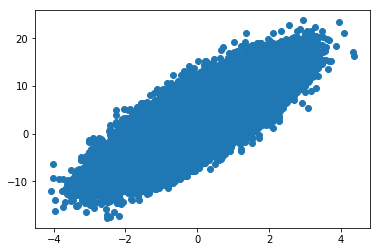
import numpy as npimport matplotlib.pyplot as plt# 准备数据m = 100000x = np.random.normal(size=m)X = x.reshape(-1,1)y = 4.*x + 3. + np.random.normal(0, 3, size=m)plt.scatter(x, y)plt.show()
def J(theta, X_b, y):try:return np.sum((y - X_b.dot(theta)) ** 2) / len(y)except:return float('inf')def dJ(theta, X_b, y):return X_b.T.dot(X_b.dot(theta) - y) * 2. / len(y)def gradient_descent(X_b, y, initial_theta, eta, n_iters=1e4, epsilon=1e-8):theta = initial_thetacur_iter = 0while cur_iter < n_iters:gradient = dJ(theta, X_b, y)last_theta = thetatheta = theta - eta * gradientif (abs(J(theta, X_b, y) - J(last_theta, X_b, y)) < epsilon):breakcur_iter += 1return theta%%time # Wall time: 884 msX_b = np.hstack([np.ones((len(X), 1)), X])initial_theta = np.zeros(X_b.shape[1])eta = 0.01theta = gradient_descent(X_b, y, initial_theta, eta) # array([3.00317559, 4.01432714])
def dJ_sgd(theta, X_b_i, y_i):return 2 * X_b_i.T.dot(X_b_i.dot(theta) - y_i)def sgd(X_b, y, initial_theta, n_iters):t0, t1 = 5, 50def learning_rate(t):return t0 / (t + t1)theta = initial_thetafor cur_iter in range(n_iters):rand_i = np.random.randint(len(X_b))gradient = dJ_sgd(theta, X_b[rand_i], y[rand_i])theta = theta - learning_rate(cur_iter) * gradientreturn theta%%time # Wall time: 226 msX_b = np.hstack([np.ones((len(X), 1)), X])initial_theta = np.zeros(X_b.shape[1])theta = sgd(X_b, y, initial_theta, n_iters=m//3)theta # array([ 3.04732375, 4.03214249])
封装SGD模型
import numpy as npfrom .metrics import r2_scoreclass LinearRegression:def __init__(self):"""初始化Linear Regression模型"""self.coef_ = Noneself.intercept_ = Noneself._theta = Nonedef fit_normal(self, X_train, y_train):"""根据训练数据集X_train, y_train训练Linear Regression模型"""assert X_train.shape[0] == y_train.shape[0], \"the size of X_train must be equal to the size of y_train"X_b = np.hstack([np.ones((len(X_train), 1)), X_train])self._theta = np.linalg.inv(X_b.T.dot(X_b)).dot(X_b.T).dot(y_train)self.intercept_ = self._theta[0]self.coef_ = self._theta[1:]return selfdef fit_bgd(self, X_train, y_train, eta=0.01, n_iters=1e4):"""根据训练数据集X_train, y_train, 使用梯度下降法训练Linear Regression模型"""assert X_train.shape[0] == y_train.shape[0], \"the size of X_train must be equal to the size of y_train"def J(theta, X_b, y):try:return np.sum((y - X_b.dot(theta)) ** 2) / len(y)except:return float('inf')def dJ(theta, X_b, y):return X_b.T.dot(X_b.dot(theta) - y) * 2. / len(y)def gradient_descent(X_b, y, initial_theta, eta, n_iters=1e4, epsilon=1e-8):theta = initial_thetacur_iter = 0while cur_iter < n_iters:gradient = dJ(theta, X_b, y)last_theta = thetatheta = theta - eta * gradientif (abs(J(theta, X_b, y) - J(last_theta, X_b, y)) < epsilon):breakcur_iter += 1return thetaX_b = np.hstack([np.ones((len(X_train), 1)), X_train])initial_theta = np.zeros(X_b.shape[1])self._theta = gradient_descent(X_b, y_train, initial_theta, eta, n_iters)self.intercept_ = self._theta[0]self.coef_ = self._theta[1:]return selfdef fit_sgd(self, X_train, y_train, n_iters=50, t0=5, t1=50):"""根据训练数据集X_train, y_train, 使用梯度下降法训练Linear Regression模型"""assert X_train.shape[0] == y_train.shape[0], \"the size of X_train must be equal to the size of y_train"assert n_iters >= 1def dJ_sgd(theta, X_b_i, y_i):return X_b_i * (X_b_i.dot(theta) - y_i) * 2.def sgd(X_b, y, initial_theta, n_iters=5, t0=5, t1=50):def learning_rate(t):return t0 / (t + t1)theta = initial_thetam = len(X_b)for i_iter in range(n_iters):indexes = np.random.permutation(m)X_b_new = X_b[indexes,:]y_new = y[indexes]for i in range(m):gradient = dJ_sgd(theta, X_b_new[i], y_new[i])theta = theta - learning_rate(i_iter * m + i) * gradientreturn thetaX_b = np.hstack([np.ones((len(X_train), 1)), X_train])initial_theta = np.random.randn(X_b.shape[1])self._theta = sgd(X_b, y_train, initial_theta, n_iters, t0, t1)self.intercept_ = self._theta[0]self.coef_ = self._theta[1:]return selfdef predict(self, X_predict):"""给定待预测数据集X_predict,返回表示X_predict的结果向量"""assert self.intercept_ is not None and self.coef_ is not None, \"must fit before predict!"assert X_predict.shape[1] == len(self.coef_), \"the feature number of X_predict must be equal to X_train"X_b = np.hstack([np.ones((len(X_predict), 1)), X_predict])return X_b.dot(self._theta)def score(self, X_test, y_test):"""根据测试数据集 X_test 和 y_test 确定当前模型的准确度"""y_predict = self.predict(X_test)return r2_score(y_test, y_predict)def __repr__(self):return "LinearRegression()"
模拟实现封装的SGD模型
模拟数据
import numpy as npimport matplotlib.pyplot as pltm = 100000x = np.random.normal(size=m)X = x.reshape(-1,1)y = 4.*x + 3. + np.random.normal(0, 3, size=m)from playML.LinearRegression import LinearRegressionlin_reg = LinearRegression()lin_reg.fit_bgd(X, y)print(lin_reg.intercept_, lin_reg.coef_) # 3.01644183437 [ 3.99995653]lin_reg = LinearRegression()lin_reg.fit_sgd(X, y, n_iters=2)print(lin_reg.intercept_, lin_reg.coef_) # 2.99558568395 [ 4.02610767]
数据归一化
梯度下降是一种搜索算法,过程中涉及各个特征,这就导致了每次的梯度值的大小受各个特征数值规模的影响,因此把数据归一化可以达到大大减小每次梯度值的效果,从而加速梯度下降。
真实实现封装的SGD模型
真实数据
from sklearn import datasets# 准备数据boston = datasets.load_boston()X = boston.datay = boston.targetX = X[y < 50.0]y = y[y < 50.0]# 数据预处理## 数据分割:训练集、测试集from playML.model_selection import train_test_splitX_train, X_test, y_train, y_test = train_test_split(X, y, seed=666)## 数据归一化from sklearn.preprocessing import StandardScalerstandardScaler = StandardScaler()standardScaler.fit(X_train)X_train_standard = standardScaler.transform(X_train)X_test_standard = standardScaler.transform(X_test)# 建模from playML.LinearRegression import LinearRegressionlin_reg = LinearRegression()%time lin_reg.fit_sgd(X_train_standard, y_train, n_iters=2) # Wall time: 3.99 mslin_reg.score(X_test_standard, y_test) # 0.78651716204682975## 调整n_iters%time lin_reg.fit_sgd(X_train_standard, y_train, n_iters=50) # Wall time: 78.8 mslin_reg.score(X_test_standard, y_test) # 0.8085728716573835%time lin_reg.fit_sgd(X_train_standard, y_train, n_iters=100) # Wall time: 157 mslin_reg.score(X_test_standard, y_test) # 0.8129484613272351
scikit-learn中的SGD
from sklearn.linear_model import SGDRegressorsgd_reg = SGDRegressor()%time sgd_reg.fit(X_train_standard, y_train) # Wall time: 185 mssgd_reg.score(X_test_standard, y_test) # 0.8047845970157302sgd_reg = SGDRegressor(n_iter=50)%time sgd_reg.fit(X_train_standard, y_train) # Wall time: 1.99 mssgd_reg.score(X_test_standard, y_test) # 0.8119907393187841

若有收获,就点个赞吧
0 人点赞
