4.6 案例：泰坦尼克号乘客生存预测

1 泰坦尼克号数据

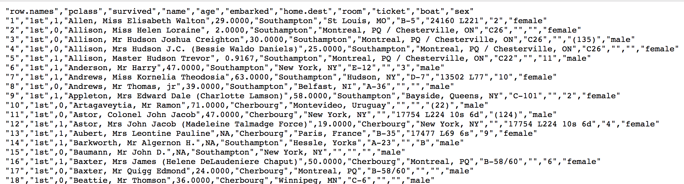
在泰坦尼克号和titanic2数据帧描述泰坦尼克号上的个别乘客的生存状态。这里使用的数据集是由各种研究人员开始的。其中包括许多研究人员创建的旅客名单，由Michael A. Findlay编辑。我们提取的数据集中的特征是票的类别，存活，乘坐班，年龄，登陆，home.dest，房间，票，船和性别。

数据：http://biostat.mc.vanderbilt.edu/wiki/pub/Main/DataSets/titanic.txt

经过观察数据得到:

• 1 乘坐班是指乘客班（1，2，3），是社会经济阶层的代表。

• 2 其中age数据存在缺失。

  2 步骤分析

• 1.获取数据

• 2.数据基本处理
  • 2.1 确定特征值,目标值
  • 2.2 缺失值处理
  • 2.3 数据集划分
• 3.特征工程(字典特征抽取)
• 4.机器学习(决策树)

• 5.模型评估

  3 代码过程

• 导入需要的模块

  import pandas as pd
  import numpy as np
  from sklearn.feature_extraction import DictVectorizer
  from sklearn.model_selection import train_test_split
  from sklearn.tree import DecisionTreeClassifier, export_graphviz

• 1.获取数据

  # 1、获取数据
  titan = pd.read_csv("http://biostat.mc.vanderbilt.edu/wiki/pub/Main/DataSets/titanic.txt")

  2.数据基本处理

• 2.1 确定特征值,目标值

  x = titan[["pclass", "age", "sex"]]
  y = titan["survived"]

• 2.2 缺失值处理

  # 缺失值需要处理，将特征当中有类别的这些特征进行字典特征抽取
  x['age'].fillna(x['age'].mean(), inplace=True)

• 2.3 数据集划分

  x_train, x_test, y_train, y_test = train_test_split(x, y, random_state=22)

• 3.特征工程(字典特征抽取)

特征中出现类别符号，需要进行one-hot编码处理(DictVectorizer)

x.to_dict(orient=”records”) 需要将数组特征转换成字典数据

# 对于x转换成字典数据x.to_dict(orient="records")
# [{"pclass": "1st", "age": 29.00, "sex": "female"}, {}]
transfer = DictVectorizer(sparse=False)
x_train = transfer.fit_transform(x_train.to_dict(orient="records"))
x_test = transfer.fit_transform(x_test.to_dict(orient="records"))

• 4.决策树模型训练和模型评估

决策树API当中，如果没有指定max_depth那么会根据信息熵的条件直到最终结束。这里我们可以指定树的深度来进行限制树的大小

# 4.机器学习(决策树)
estimator = DecisionTreeClassifier(criterion="entropy", max_depth=5)
estimator.fit(x_train, y_train)
# 5.模型评估
estimator.score(x_test, y_test)
estimator.predict(x_test)

决策树的结构是可以直接显示

3 决策树可视化

3.1 保存树的结构到dot文件

• sklearn.tree.export_graphviz() 该函数能够导出DOT格式

  • tree.export_graphviz(estimator,out_file=’tree.dot’,feature_names=[‘’,’’])

    export_graphviz(estimator, out_file="./data/tree.dot", feature_names=['age', 'pclass=1st', 'pclass=2nd', 'pclass=3rd', '女性', '男性'])

    dot文件当中的内容如下

    digraph Tree {
    node [shape=box] ;
    0 [label="petal length (cm) <= 2.45\nentropy = 1.584\nsamples = 112\nvalue = [39, 37, 36]"] ;
    1 [label="entropy = 0.0\nsamples = 39\nvalue = [39, 0, 0]"] ;
    0 -> 1 [labeldistance=2.5, labelangle=45, headlabel="True"] ;
    2 [label="petal width (cm) <= 1.75\nentropy = 1.0\nsamples = 73\nvalue = [0, 37, 36]"] ;
    0 -> 2 [labeldistance=2.5, labelangle=-45, headlabel="False"] ;
    3 [label="petal length (cm) <= 5.05\nentropy = 0.391\nsamples = 39\nvalue = [0, 36, 3]"] ;
    2 -> 3 ;
    4 [label="sepal length (cm) <= 4.95\nentropy = 0.183\nsamples = 36\nvalue = [0, 35, 1]"] ;
    3 -> 4 ;
    5 [label="petal length (cm) <= 3.9\nentropy = 1.0\nsamples = 2\nvalue = [0, 1, 1]"] ;
    4 -> 5 ;
    6 [label="entropy = 0.0\nsamples = 1\nvalue = [0, 1, 0]"] ;
    5 -> 6 ;
    7 [label="entropy = 0.0\nsamples = 1\nvalue = [0, 0, 1]"] ;
    5 -> 7 ;
    8 [label="entropy = 0.0\nsamples = 34\nvalue = [0, 34, 0]"] ;
    4 -> 8 ;
    9 [label="petal width (cm) <= 1.55\nentropy = 0.918\nsamples = 3\nvalue = [0, 1, 2]"] ;
    3 -> 9 ;
    10 [label="entropy = 0.0\nsamples = 2\nvalue = [0, 0, 2]"] ;
    9 -> 10 ;
    11 [label="entropy = 0.0\nsamples = 1\nvalue = [0, 1, 0]"] ;
    9 -> 11 ;
    12 [label="petal length (cm) <= 4.85\nentropy = 0.191\nsamples = 34\nvalue = [0, 1, 33]"] ;
    2 -> 12 ;
    13 [label="entropy = 0.0\nsamples = 1\nvalue = [0, 1, 0]"] ;
    12 -> 13 ;
    14 [label="entropy = 0.0\nsamples = 33\nvalue = [0, 0, 33]"] ;
    12 -> 14 ;
    }

    那么这个结构不能看清结构，所以可以在一个网站上显示

    3.2 网站显示结构

• http://webgraphviz.com/将dot文件内容复制到该网站当中显示

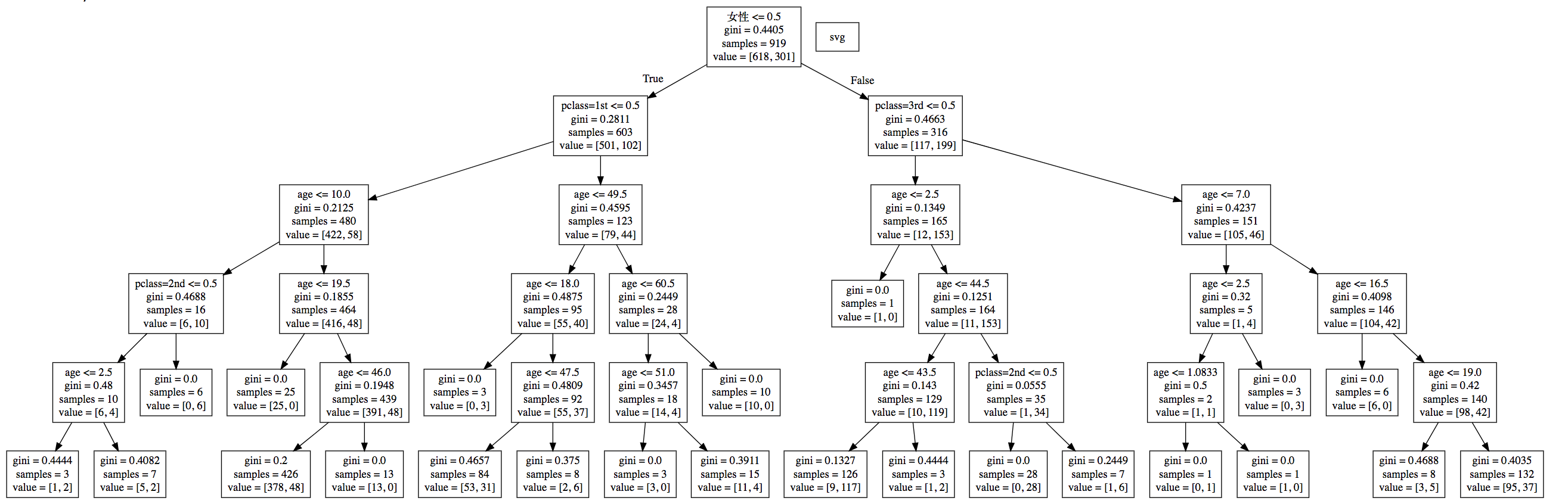
  3.5 决策树总结

• 优点：

  • 简单的理解和解释，树木可视化。
• 缺点：
  • 决策树学习者可以创建不能很好地推广数据的过于复杂的树,容易发生过拟合。
• 改进：
  • 减枝cart算法
  • 随机森林（集成学习的一种）

注：企业重要决策，由于决策树很好的分析能力，在决策过程应用较多， 可以选择特征