PyTorch 深度学习实践 第3讲

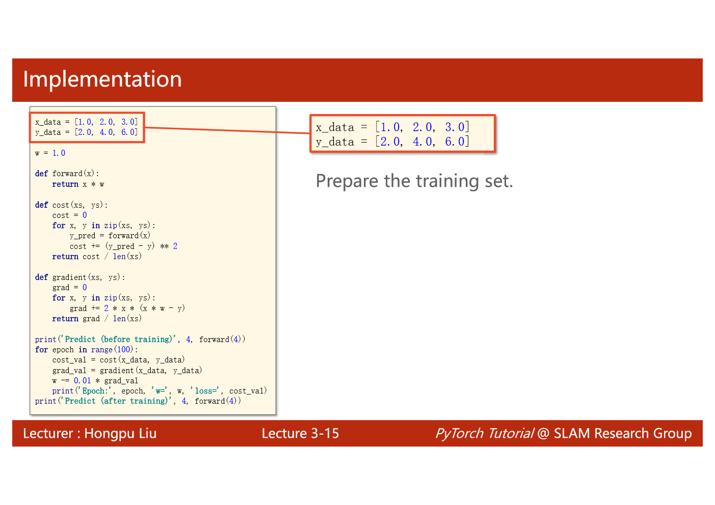
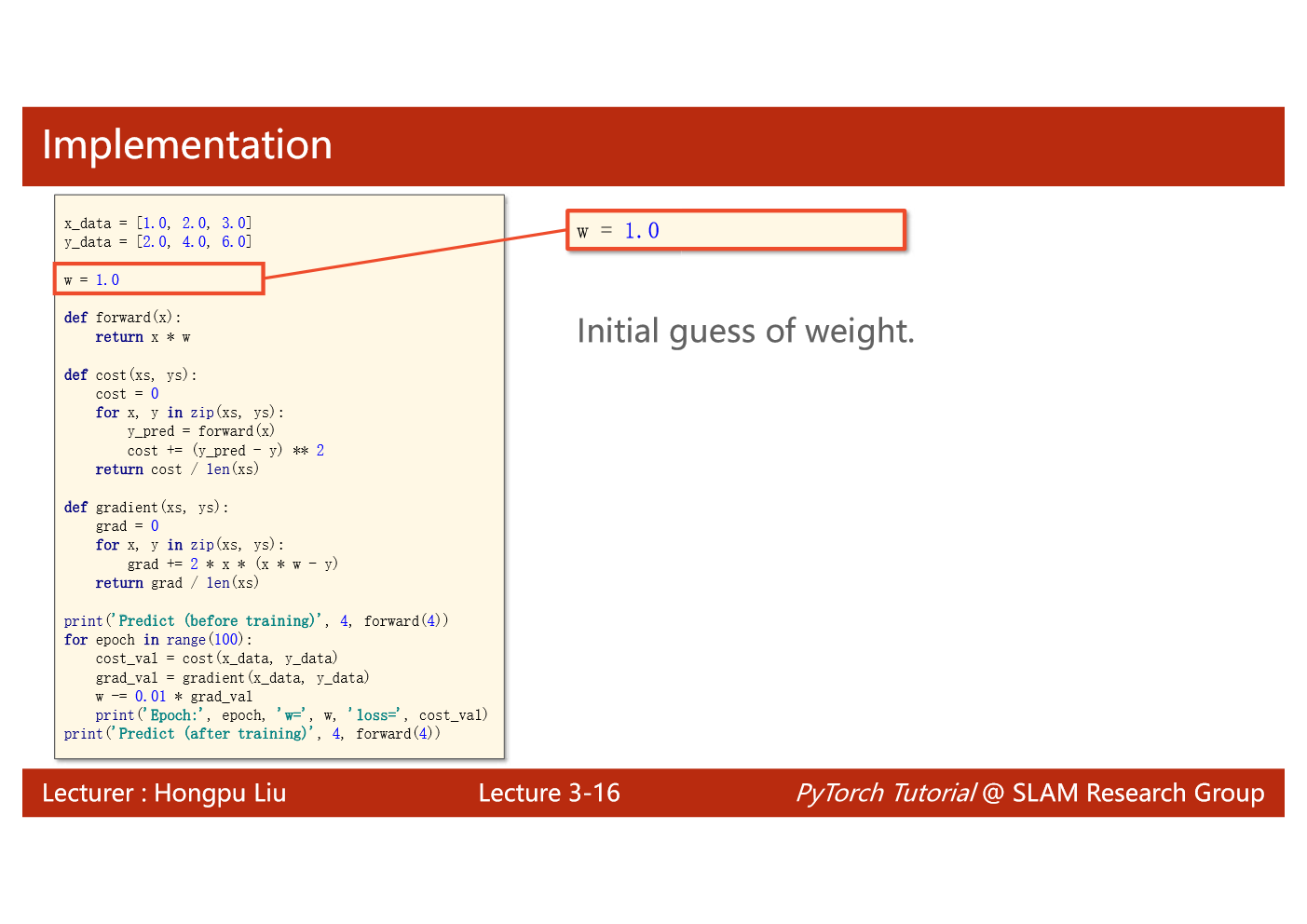
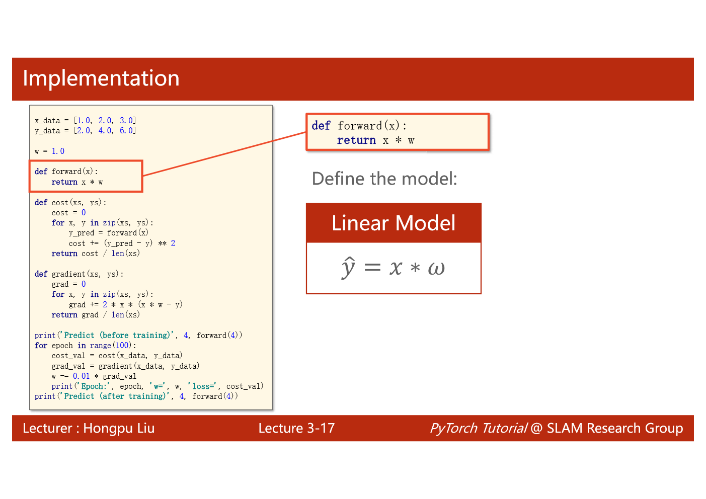
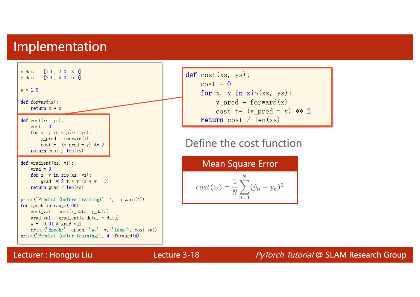
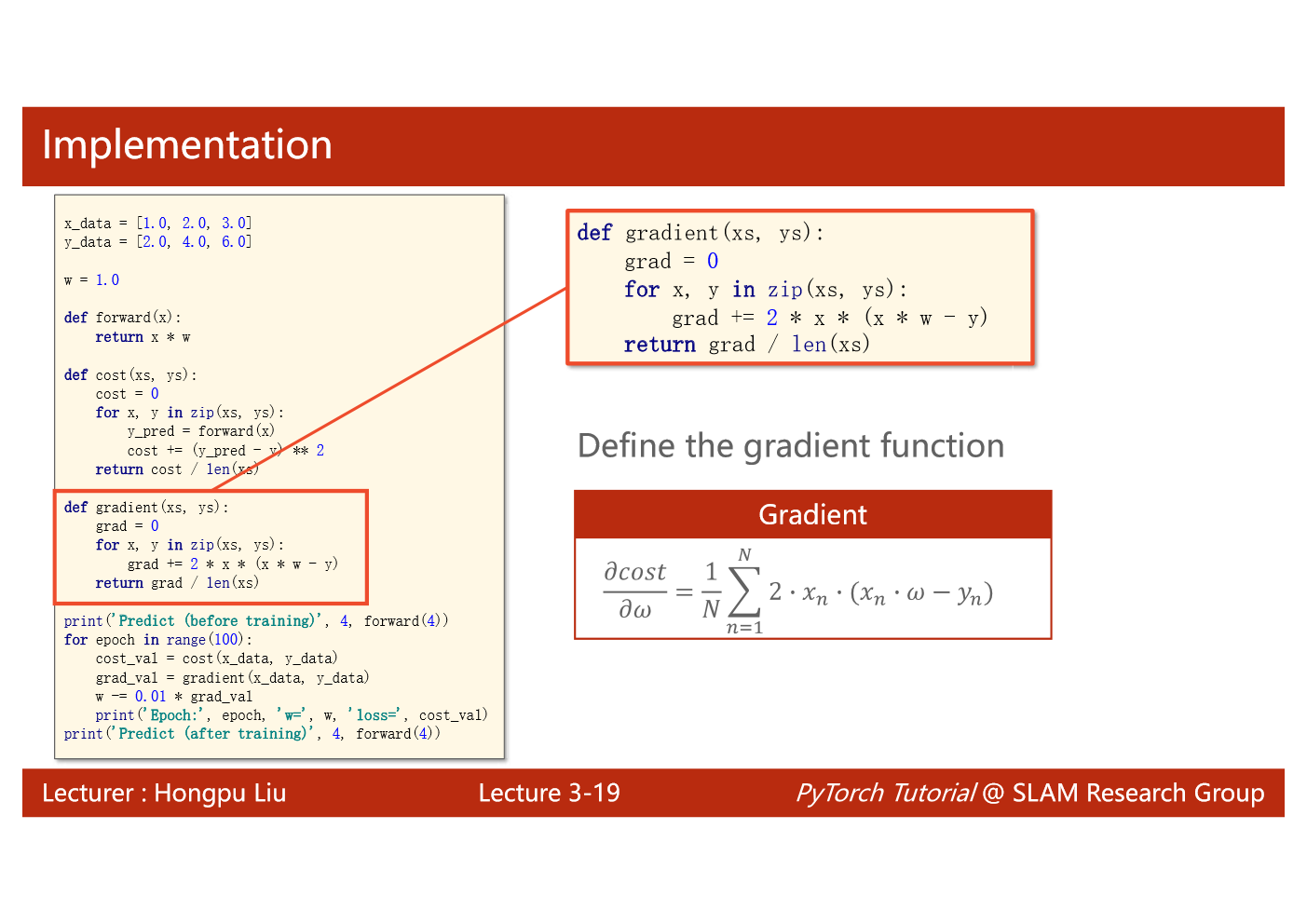
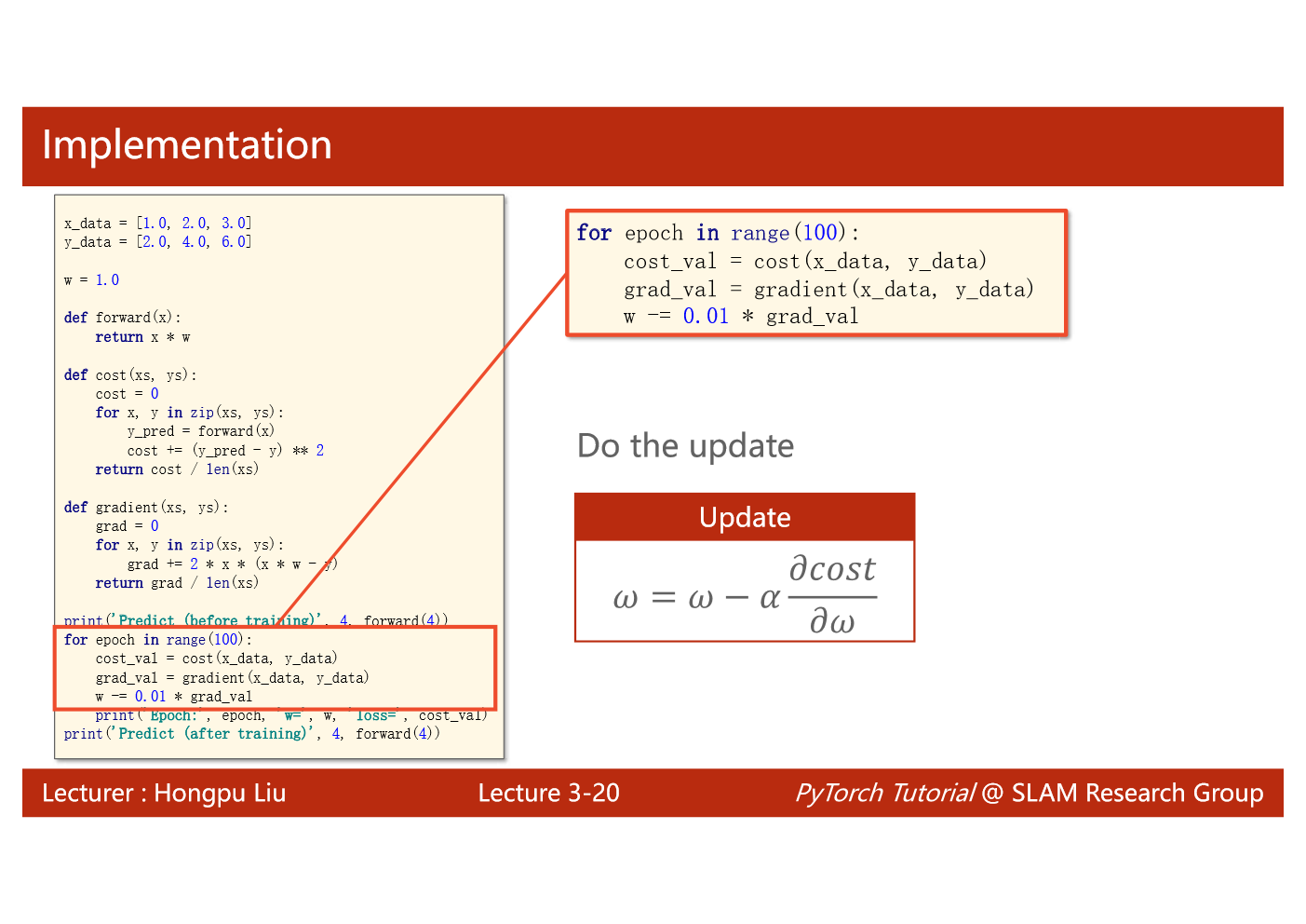
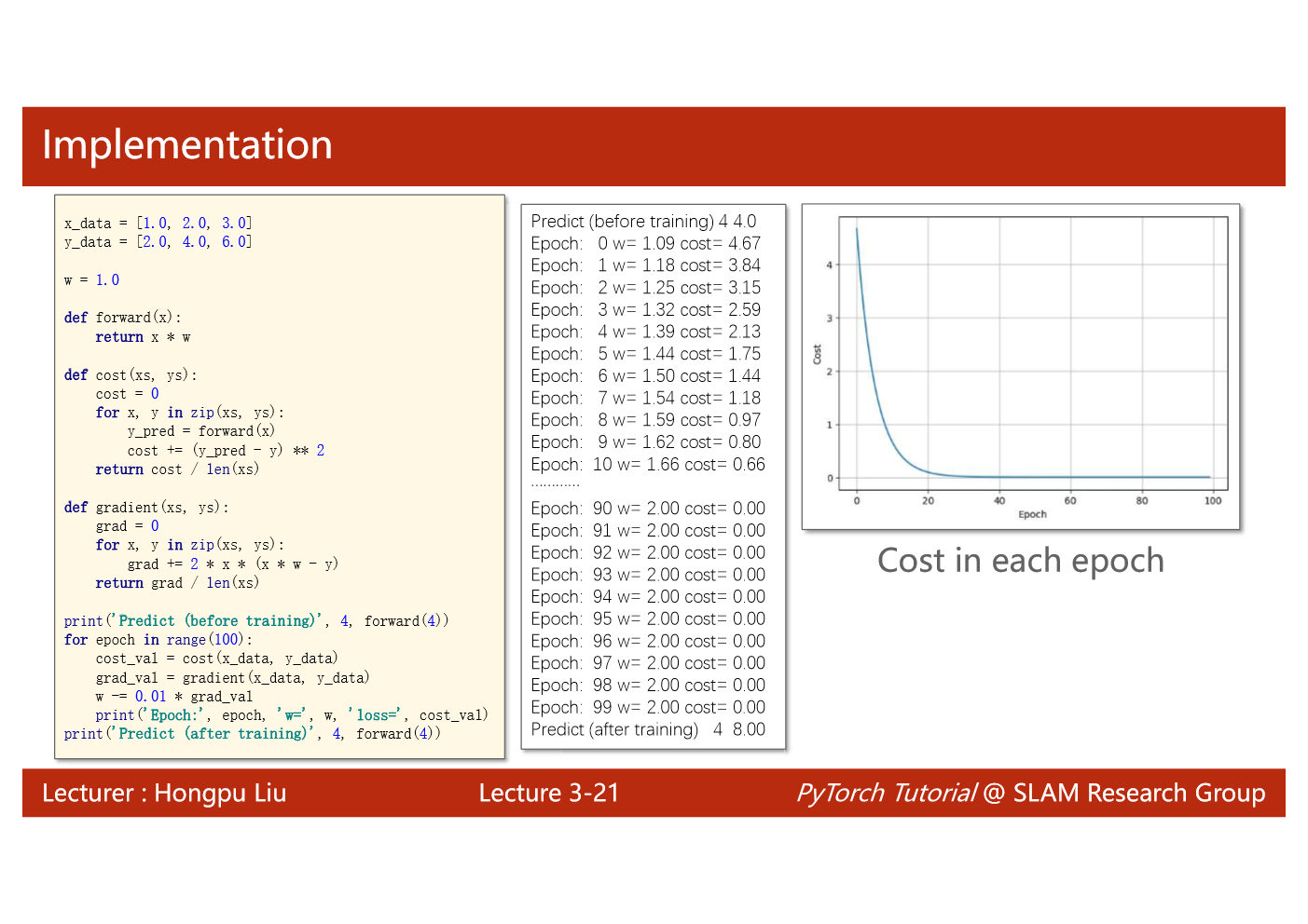
import matplotlib.pyplot as plt
# prepare the training set
x_data = [1.0, 2.0, 3.0]
y_data = [2.0, 4.0, 6.0]
# initial guess of weight 
w = 1.0
# define the model linear model y = w*x
def forward(x):
    return x*w
#define the cost function MSE 
def cost(xs, ys):
    cost = 0
    for x, y in zip(xs,ys):
        y_pred = forward(x)
        cost += (y_pred - y)**2
    return cost / len(xs)
# define the gradient function  gd
def gradient(xs,ys):
    grad = 0
    for x, y in zip(xs,ys):
        grad += 2*x*(x*w - y)
    return grad / len(xs)
epoch_list = []
cost_list = []
print('predict (before training)', 4, forward(4))
for epoch in range(100):
    cost_val = cost(x_data, y_data)
    grad_val = gradient(x_data, y_data)
    w-= 0.01 * grad_val  # 0.01 learning rate
    print('epoch:', epoch, 'w=', w, 'loss=', cost_val)
    epoch_list.append(epoch)
    cost_list.append(cost_val)
print('predict (after training)', 4, forward(4))
plt.plot(epoch_list,cost_list)
plt.ylabel('cost')
plt.xlabel('epoch')
plt.show()

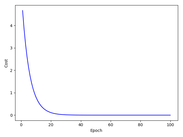
# Numpy
import numpy
# For plotting
import matplotlib.pyplot as plt
from matplotlib.pyplot import figure
def forward(w, x):
    return x * w
def cost(x_cor, y_cor, w):
    y_hat = forward(w, x_cor)
    loss = (y_hat - y_cor) ** 2
    return loss.sum() / len(x_cor)
def gradient(x_cor, y_cor, w):
    grad = 2 * x_cor * (w * x_cor - y_cor)
    return grad.sum() / len(x_cor)
x_data = numpy.array([1.0, 2.0, 3.0])
y_data = numpy.array([2.0, 4.0, 6.0])
num_epochs = 100
lr = 0.01
w_train = numpy.array([1.0])
epoch_cor = []
loss_cor = []
for epoch in range(num_epochs):
    mse_loss = cost(x_data, y_data, w_train)
    loss_cor.append(mse_loss)
    w_train -= lr * gradient(x_data, y_data, w_train)
    epoch_cor.append(epoch + 1)
plt.figure()
plt.plot(epoch_cor, loss_cor, c='b')
plt.xlabel('Epoch')
plt.ylabel('Cost')
plt.show()

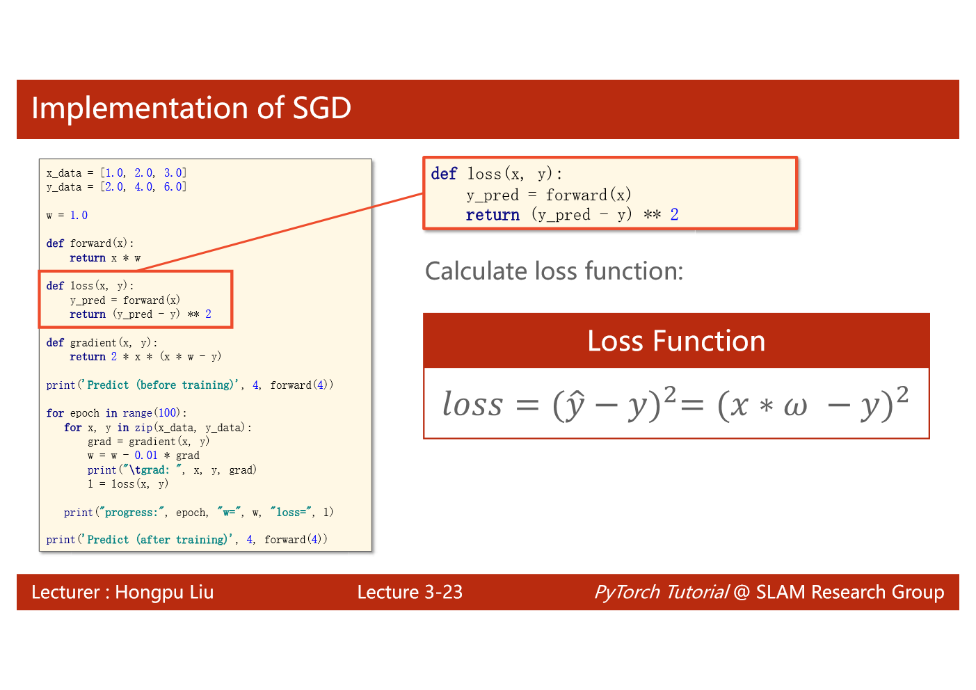
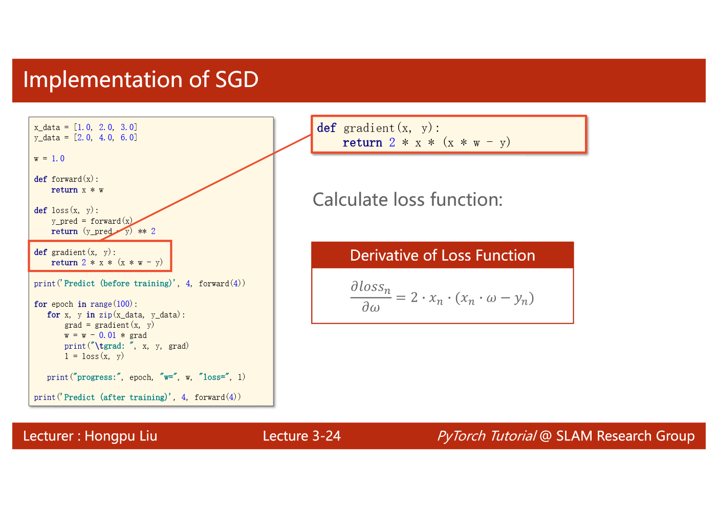
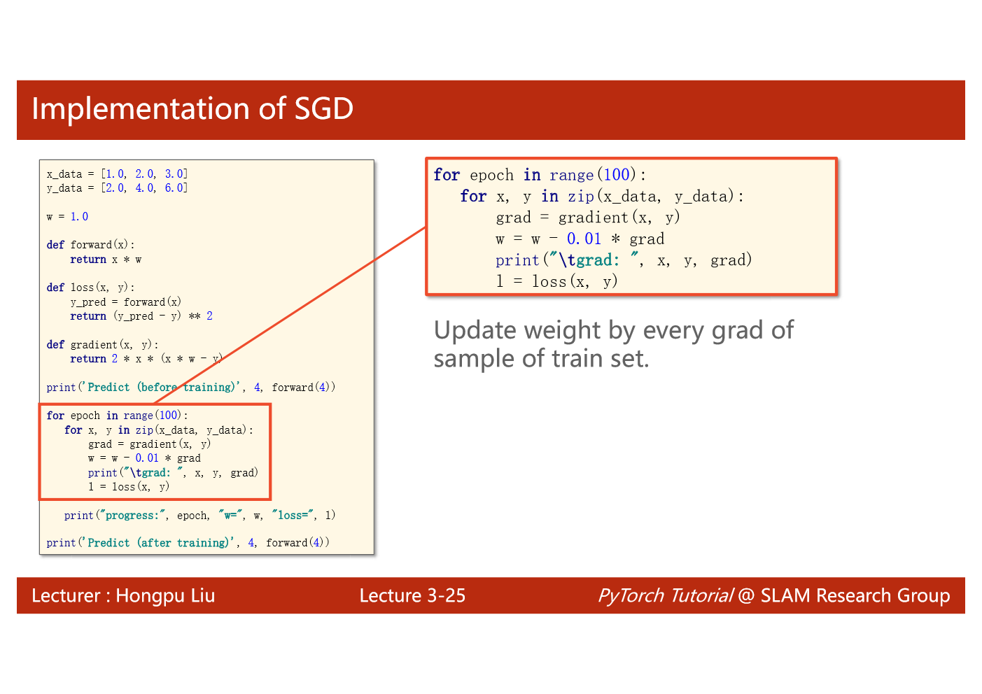
import matplotlib.pyplot as plt
x_data = [1.0, 2.0, 3.0]
y_data = [2.0, 4.0, 6.0]
w = 1.0
def forward(x):
    return x*w
# calculate loss function
def loss(x, y):
    y_pred = forward(x)
    return (y_pred - y)**2
# define the gradient function  sgd
def gradient(x, y):
    return 2*x*(x*w - y)
epoch_list = []
loss_list = []
print('predict (before training)', 4, forward(4))
for epoch in range(100):
    for x,y in zip(x_data, y_data):
        grad = gradient(x,y)
        w = w - 0.01*grad    # update weight by every grad of sample of training set
        print("\tgrad:", x, y,grad)
        l = loss(x,y)
    print("progress:",epoch,"w=",w,"loss=",l)
    epoch_list.append(epoch)
    loss_list.append(l)
print('predict (after training)', 4, forward(4))
plt.plot(epoch_list,loss_list)
plt.ylabel('loss')
plt.xlabel('epoch')
plt.show()

随机梯度下降法在神经网络中被证明是有效的。效率较低(时间复杂度较高)，学习性能较好。

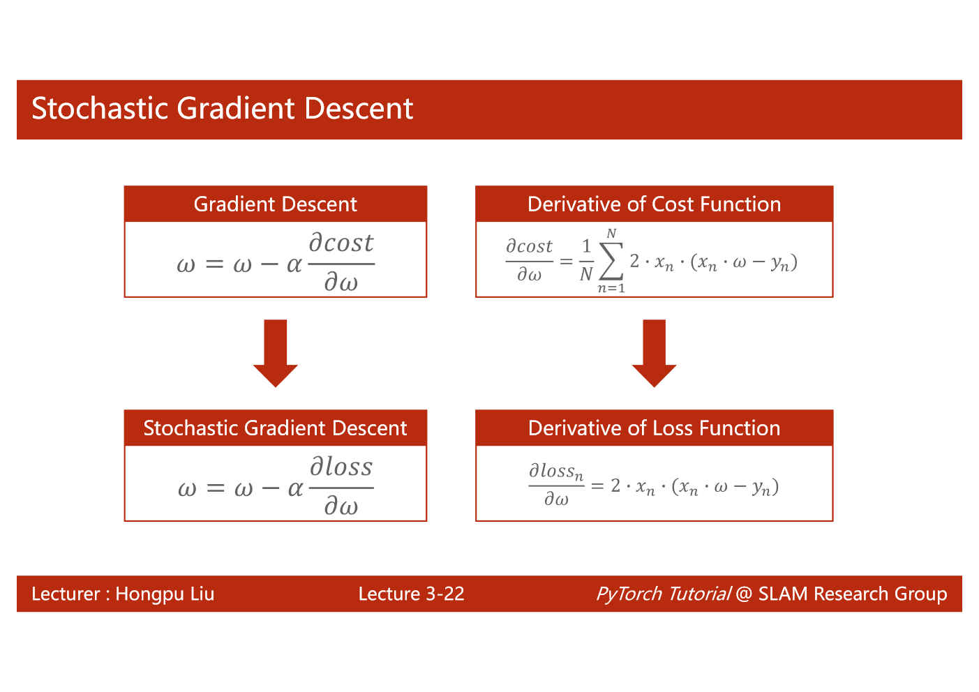
随机梯度下降法和梯度下降法的主要区别在于：

1、损失函数由cost()更改为loss()。cost是计算所有训练数据的损失，loss是计算一个训练函数的损失。对应于源代码则是少了两个for循环。
2、梯度函数gradient()由计算所有训练数据的梯度更改为计算一个训练数据的梯度。
3、本算法中的随机梯度主要是指，每次拿一个训练数据来训练，然后更新梯度参数。本算法中梯度总共更新100(epoch)x3 = 300次。梯度下降法中梯度总共更新100(epoch)次。

综合梯度下降和随机梯度下降算法，折中：batch（mini-patch）