基于 Perception 感知器算法实现鸢尾花二分类
import numpy as npimport pandas as pd
data = pd.read_csv(r"dataset/iris.arff.csv", header=0)# data.head(10)# data.tail(10)# print(data.sample(10))# data = data.drop("Id",axis=1) # 删除列print(len(data))if data.duplicated().any(): # 重复值data.drop_duplicates(inplace=True) #删除重复值print(len(data))display(data["class"].value_counts()) # 计算每个类别的数量# 因为感知器映射结果为1和-1,所以这里这也处理data["class"] = data["class"].map({"Iris-versicolor":0,"Iris-setosa":-1,"Iris-virginica":1}) # 类别名称映射为数字data = data[data["class"]!=0]len(data)
150
147
Iris-versicolor 50
Iris-virginica 49
Iris-setosa 48
Name: class, dtype: int64
Out[8]: 97
class Perception:'''感知器算法实现。二分类'''def __init__(self, learning_rate, times):'''初始化Parameters-----learning_rate: float 学习率times: int 迭代次数'''self.learning_rate = learning_rateself.times = timesdef step(self, z):'''阶跃函数Paraammeters-----z: 数组类型(或者是标量) 阶跃函数参数。将z映射为1或者-1Return-----value: int z>0返回1.z<0返回1'''return np.where(z>0, 1,-1) # 一步实现对数值或者数组的计算返回def fit(self, X, y):'''训练Parameters-----X: 特征矩阵,可以是List也可以是Ndarray,形状为: [样本数量,特征数量]y: 标签数组'''X = np.asarray(X)y = np.asarray(y)# 创建权重向量。初始值为0。长度比特征多1.多出的是截距self.w_ = np.zeros(1 + X.shape[1])# 创建损失列表,用来保存每次迭代后的损失值self.loss_ = []for i in range(self.times):# 感知器与逻辑回归的区别:逻辑回归中。使用所有样本计算梯度来更新权重。# 而感知器是使用单个样本,依次计算梯度更新权重loss = 0for x,target in zip(X,y):# 计算预测值y_hat = self.step(np.dot(x, self.w_[1:]) + self.w_[0])# 如果预测值不等于目标值,返回1,loss+1,否则loss不增加loss += y_hat != target# 更新权重# w(j) = w(j) + 学习率 * (真实值-预测值)*x(j)self.w_[0] += self.learning_rate * (target - y_hat)self.w_[1:] += self.learning_rate * (target - y_hat) * x# 将循环累计误差值增加到误差列表中self.loss_.append(loss)def predit(self, X):'''根据参数预测Parametres:X: 特征矩阵,可以是List也可以是Ndarray,形状为: [样本数量,特征数量]Return-----value: 数组类型, 分类值[1或-1]'''return self.step(np.dot(X, self.w_[1:]) + self.w_[0])
t1 = data[data["class"]==1]t2 = data[data["class"]==-1]t1.sample(len(t1), random_state=0)t2.sample(len(t2), random_state=0)train_X = pd.concat([t1.iloc[:40,:-1], t2.iloc[:40, :-1]], axis=0)train_y = pd.concat([t1.iloc[:40,-1], t2.iloc[:40, -1]], axis=0)test_X = pd.concat([t1.iloc[40:,:-1], t2.iloc[40:, :-1]], axis=0)test_y = pd.concat([t1.iloc[40:,-1], t2.iloc[40:, -1]], axis=0)p = Perception(0.1, 10)p.fit(train_X,train_y)result = p.predit(test_X)# resultdisplay(result)display(test_y.values)display(p.w_)display(p.loss_) # 可以看出每次迭代后损失值就下降了
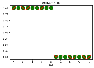
array([ 1, 1, 1, 1, 1, 1, 1, 1, 1, -1, -1, -1, -1, -1, -1, -1, -1])
array([ 1, 1, 1, 1, 1, 1, 1, 1, 1, -1, -1, -1, -1, -1, -1, -1, -1], dtype=int64)
array([-0.2 , -0.5 , -0.68, 1.56, 0.88])
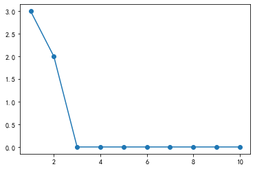
[3, 2, 0, 0, 0, 0, 0, 0, 0, 0]
import matplotlib as mplimport matplotlib.pyplot as pltmpl.rcParams["font.family"] = "SimHei"mpl.rcParams["axes.unicode_minus"] = False # 显示负号
# 绘制真实值plt.plot(test_y.values, "go", ms=15, label="真实值")plt.plot(result, "rx", ms=15, label="预测值")plt.title("感知器二分类")plt.xlabel("样本序号")plt.xlabel("类别")plt.show()
# 绘制目标函数损失值plt.plot(range(1, p.times+1), p.loss_, "o-")
[

若有收获,就点个赞吧
0 人点赞
