使用scater包进行单细胞测序分析（三）：数据降维与可视化

本次教程学习使用scater包进行单细胞转录组数据降维与常用的一些可视化方法。

• plotExpression: plot cell expression levels for one or more genes;
• plotReducedDim: plot (and/or calculate) reduced dimension coordinates;

加载所需的R包和示例数据

library(scater)
data("sc_example_counts")
data("sc_example_cell_info")
# 构建SingleCellExperiment对象
example_sce <- SingleCellExperiment(
    assays = list(counts = sc_example_counts),
    colData = sc_example_cell_info
) 
# 进行数据归一化
example_sce <- normalize(example_sce)
example_sce
## class: SingleCellExperiment 
## dim: 2000 40 
## metadata(1): log.exprs.offset
## assays(2): counts logcounts
## rownames(2000): Gene_0001 Gene_0002 ... Gene_1999 Gene_2000
## rowData names(0):
## colnames(40): Cell_001 Cell_002 ... Cell_039 Cell_040
## colData names(4): Cell Mutation_Status Cell_Cycle Treatment
## reducedDimNames(0):
## spikeNames(0):

基因表达量的可视化

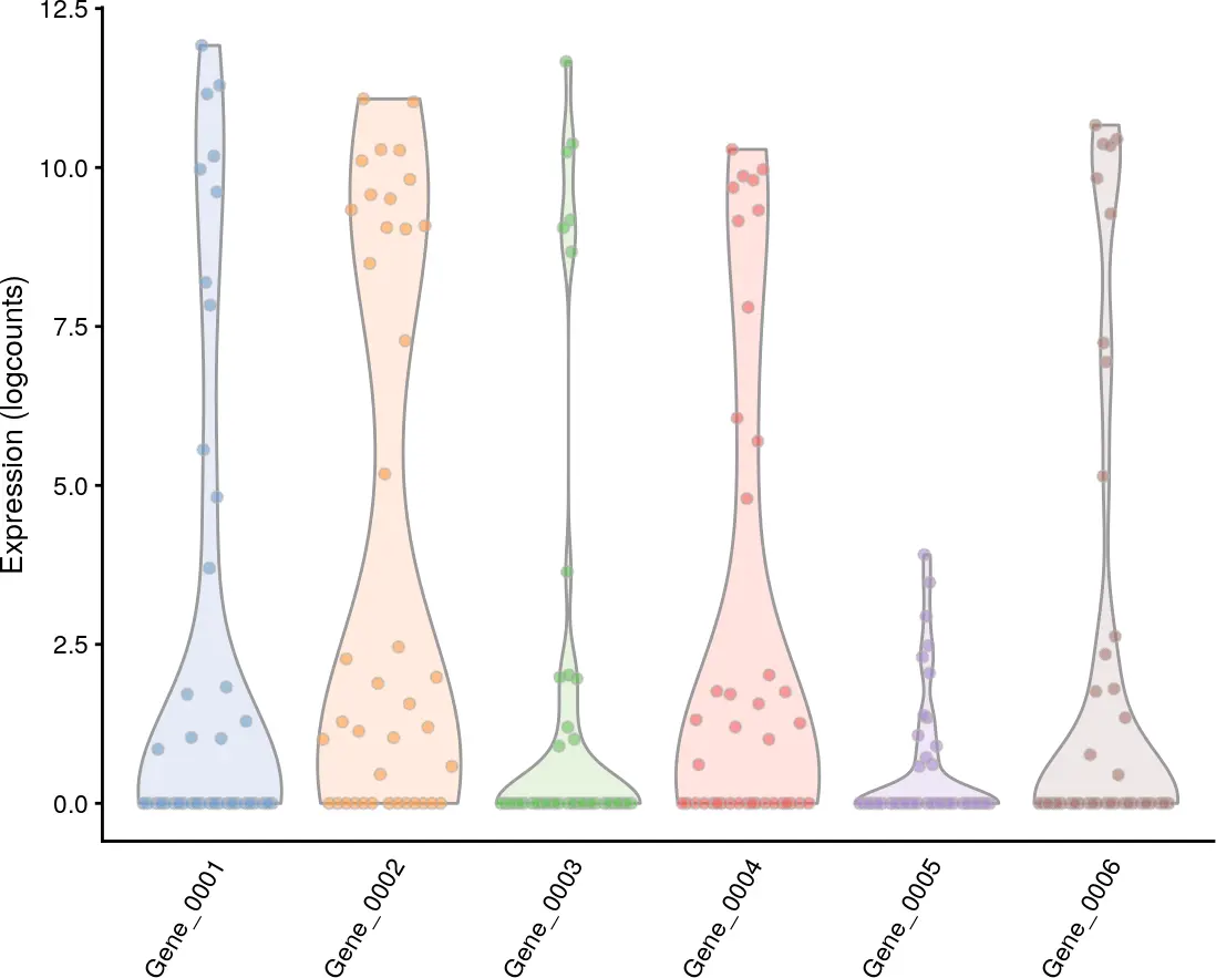
在scater包中，我们使用plotExpression函数对(特征)基因的表达量进行可视化展示。默认情况下，它使用归一化后的“logcounts”值进行可视化，我们也可以通过exprs_values参数对其进行更改。

plotExpression(example_sce, rownames(example_sce)[1:6],
    x = "Mutation_Status", exprs_values = "logcounts")

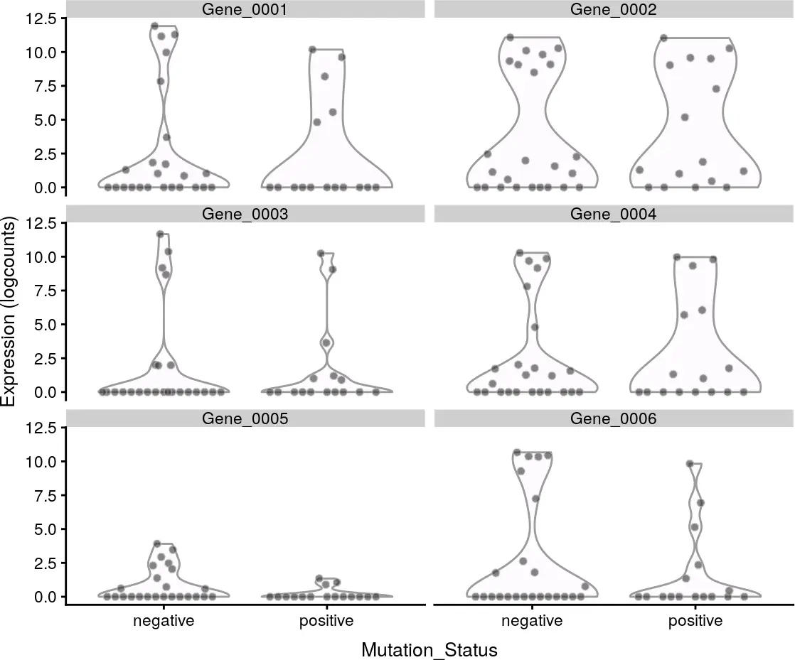
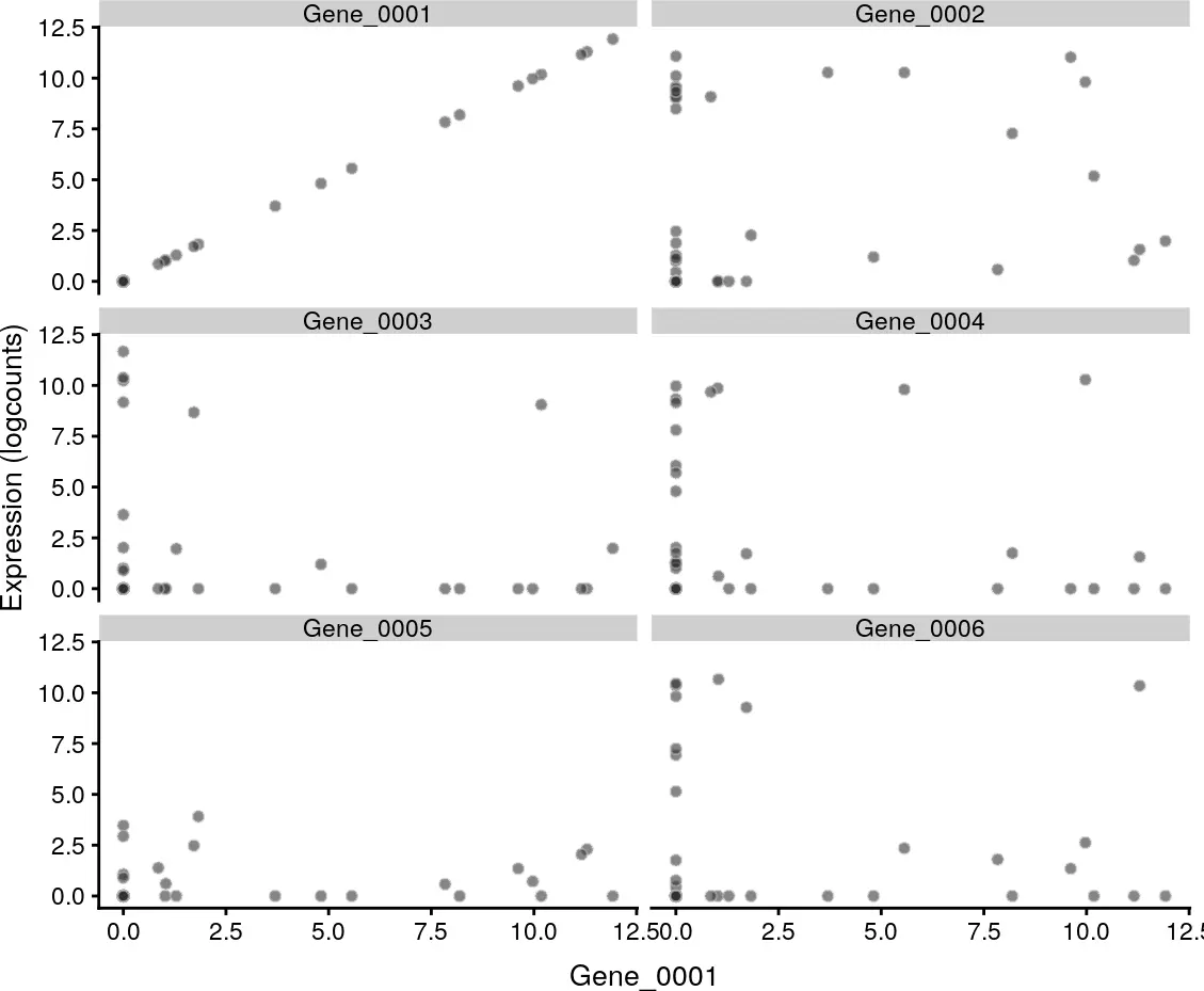
设置x参数确定在x轴上显示的协变量，它可以是列元数据中的字段，也可以是某个基因的名称。对于分类协变量，将产生如上图所示的分组小提琴图；而对于连续协变量，将在每个面板中生成散点图，如下图所示。

plotExpression(example_sce, rownames(example_sce)[1:6],
    x = "Gene_0001")

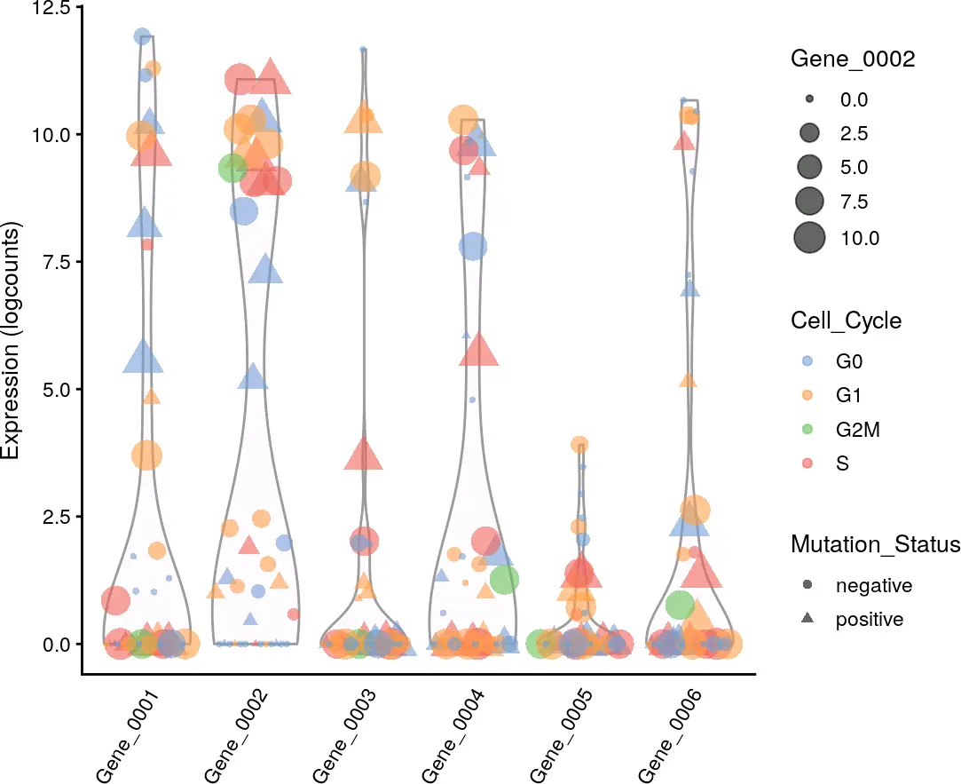
当然，我们也可以通过colour_by，shape_by和size_by等参数调整点的颜色，形状和大小。

plotExpression(example_sce, rownames(example_sce)[1:6],
    colour_by = "Cell_Cycle", shape_by = "Mutation_Status", 
    size_by = "Gene_0002")

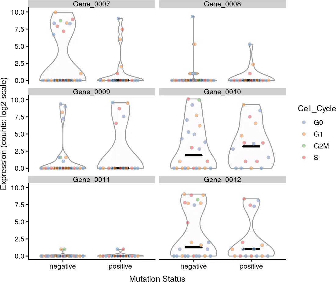
对于分类协变量x，我们还可以通过设置show_median = TRUE参数，在小提琴图上显示每组表达水平的中位数。

plotExpression(example_sce, rownames(example_sce)[7:12],
    x = "Mutation_Status", exprs_values = "counts", 
    colour = "Cell_Cycle", show_median = TRUE, 
    xlab = "Mutation Status", log = TRUE)

如果不设置x参数，plotExpression函数将直接绘制一组所选基因的表达量的小提琴图。

plotExpression(example_sce, rownames(example_sce)[1:6])

数据的降维与可视化

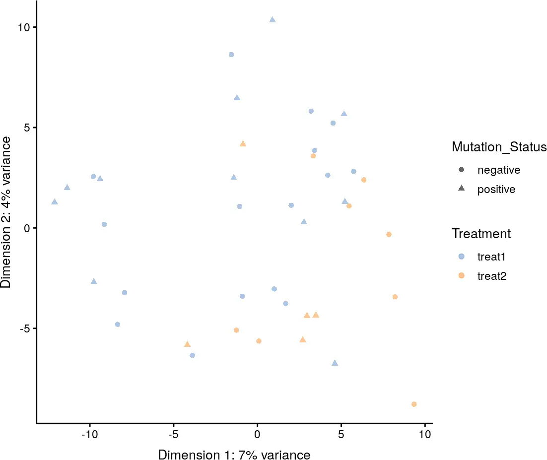
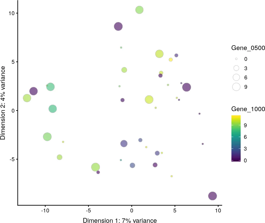
scater包可以使用多种方法（PCA, tSNE, UMAP和diffussion maps）对单细胞转录组数据进行降维处理，降维后的结果存储在reducedDims slot中，可以使用plotReducedDim函数对降维后的结果进行可视化展示，并通过use_dimred参数设置降维的方法。

使用PCA方法进行数据降维可视化

scater包使用runPCA函数进行PCA降维处理，通过plotPCA函数进行降维可视化展示，也可以使用plotReducedDim函数对PCA降维后的结果进行可视化展示。

# 使用runPCA函数进行PCA降维处理
example_sce <- runPCA(example_sce)

reducedDimNames(example_sce)
## [1] "PCA"

# 使用plotReducedDim函数对降维结果进行可视化展示，use_dimred参数设置降维的方法
plotReducedDim(example_sce, use_dimred = "PCA", 
    colour_by = "Treatment", shape_by = "Mutation_Status")

plotReducedDim(example_sce, use_dimred = "PCA", 
    colour_by = "Gene_1000", size_by = "Gene_0500")

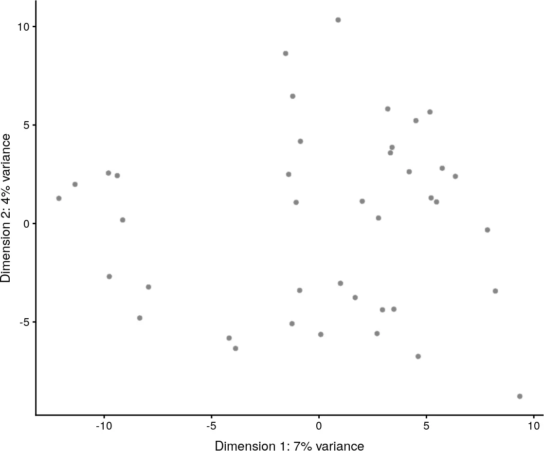
使用plotPCA函数对PCA降维的结果进行可视化展示，默认会对reduceDims slot中的PCA降维结果的前两个主成分进行可视化。

plotPCA(example_sce)

如果在使用plotPCA函数时不存在预先计算好的“PCA”结果，该函数将会自动调用runPCA函数计算PCA降维的结果。
默认情况下，runPCA函数会使用所有细胞中最高变化的500个基因的表达量的log-counts值来执行PCA降维处理，也可以通过ntop参数设置使用的高可变基因的数量。或者，通过feature_set参数设置用于PCA降维处理的一组特定基因。

example_sce2 <- runPCA(example_sce, 
    feature_set = rowData(example_sce)$is_feature_control)

plotPCA(example_sce2)

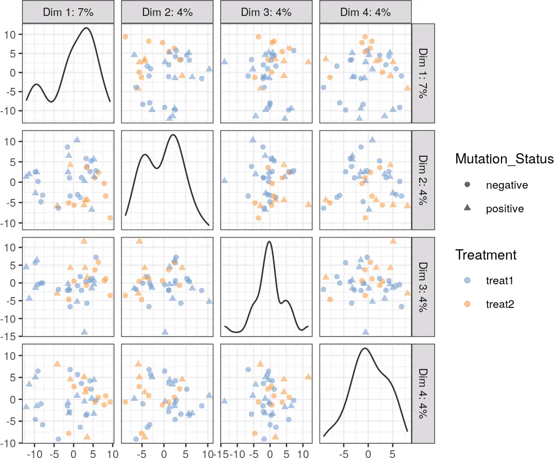
Multiple components can be plotted in a series of pairwise plots. When more than two components are plotted, the diagonal boxes in the scatter plot matrix show the density for each component.

example_sce <- runPCA(example_sce, ncomponents=20)
plotPCA(example_sce, ncomponents = 4, colour_by = "Treatment",
        shape_by = "Mutation_Status")

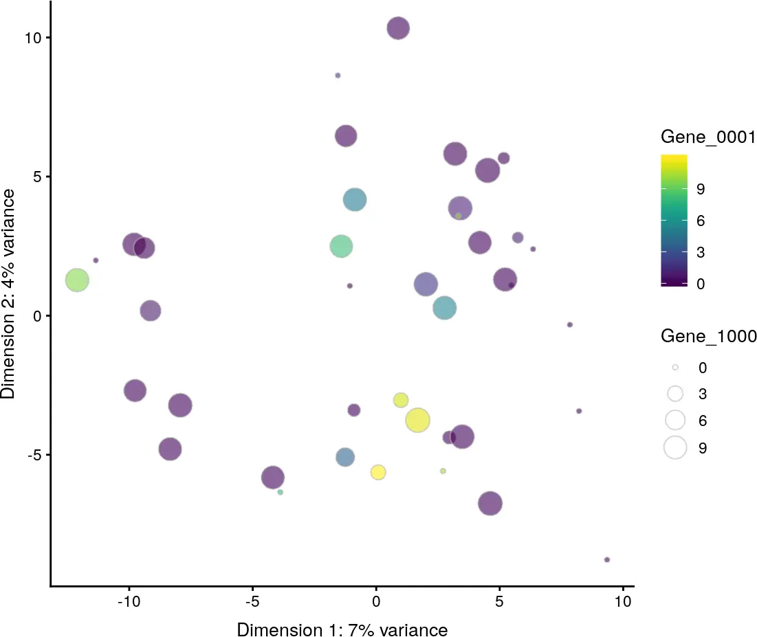
plotPCA(example_sce, colour_by = "Gene_0001", size_by = "Gene_1000")

使用tSNE方法进行数据降维可视化

t-SNE方法被广泛用于复杂的单细胞数据集的降维可视化处理，scater通过Rtsne包使用runTSNE函数进行降维处理，获得tSNE降维后的坐标信息，使用plotTSNE函数可视化tSNE降维后的结果。

# Perplexity of 10 just chosen here arbitrarily. 
set.seed(1000)
# 使用runTSNE函数进行tSNE数据降维处理
example_sce <- runTSNE(example_sce, perplexity=10)
# 使用plotTSNE函数将降维可视化展示
plotTSNE(example_sce, colour_by = "Gene_0001", size_by = "Gene_1000")

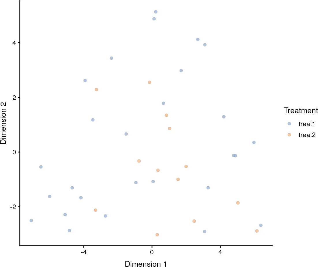
当然，我们也可以使用预先计算好的PCA降维结果作为t-SNE算法的输入，这可以使用low-rank approximation的表达矩阵提升计算的速度，也可以降低随机噪音。

set.seed(1000)
example_sce <- runTSNE(example_sce, perplexity=10, use_dimred="PCA", n_dimred=10)
plotTSNE(example_sce, colour_by="Treatment")

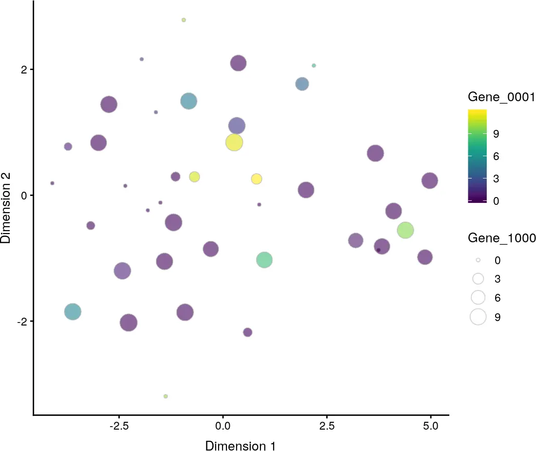
使用diffusion maps方法进行数据降维可视化

scater通过density包使用runDiffusionMap函数进行diffusion maps降维处理，并使用plotDiffusionMap函数对降维后的结果进行可视化展示。

# 使用runDiffusionMap函数进行降维处理
example_sce <- runDiffusionMap(example_sce)
使用plotDiffusionMap函数对降维结果进行可视化展示
plotDiffusionMap(example_sce, colour_by = "Gene_0001", size_by = "Gene_1000")

参考来源：http://www.bioconductor.org/packages/release/bioc/vignettes/scater/inst/doc/overview.html