scater包简介
scater是一个优秀的单细胞转录组数据分析工具包,它可以对单细胞数据进行常规的质量控制,数据的标准化与归一化,以及数据的降维与可视化分析。它主要基于SingleCellExperiment类(来自SingleCellExperiment包)来进行操作处理,因此可以与其他许多Bioconductor包(如scran,batchelor和iSEE等)相互操作。
scater包主要含有以下特性:
- Use of the
SingleCellExperimentclass as adata containerfor interoperability with a wide range of other Bioconductor packages; - Functions to import
kallistoandSalmonresults; - Simple calculation of many
quality control metricsfrom the expression data; - Many tools for
visualising scRNA-seq data, especially diagnostic plots for quality control; - Subsetting and many other methods for
filtering out problematic cells and features; - Methods for
identifying important experimental variablesandnormalising dataahead of downstream statistical analysis and modeling.
scater包的工作流程为: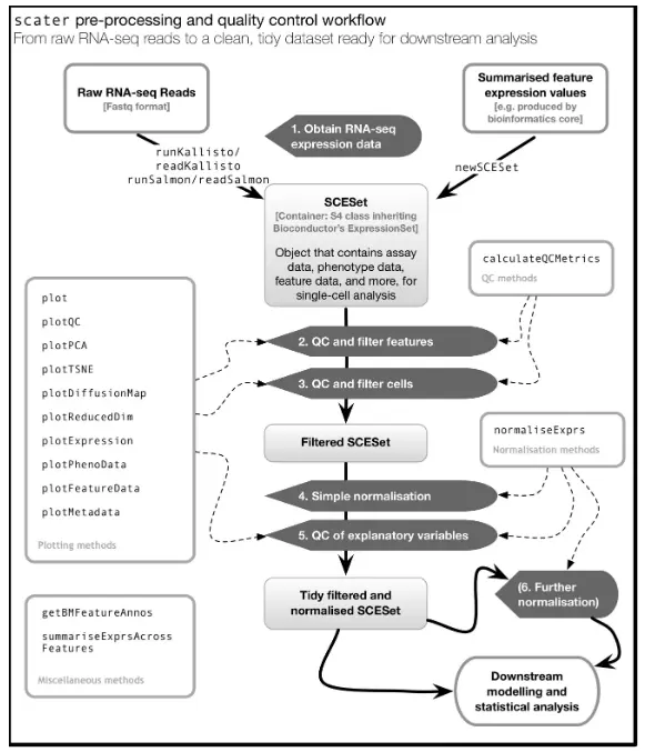
构建SingleCellExperiment对象
使用SingleCellExperiment函数导入单细胞转录组的基因表达矩阵构建一个SingleCellExperiment对象,该表达矩阵是一个行为基因,列为细胞的大型数据框。
SingleCellExperiment对象内容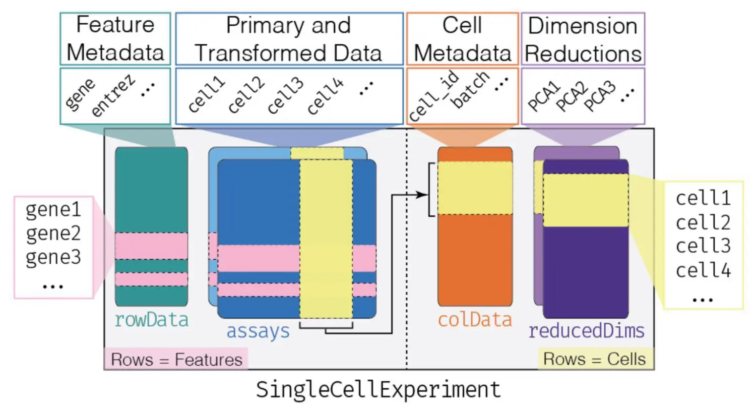
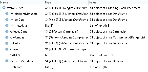
SingleCellExperiment对象常见操作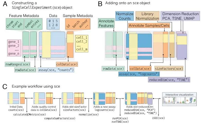
# 导入scater包library(scater)# 加载示例数据data("sc_example_counts")data("sc_example_cell_info")# 查看基因表达矩阵head(sc_example_counts)Cell_001 Cell_002 Cell_003 Cell_004 Cell_005 Cell_006 Cell_007Gene_0001 0 123 2 0 0 0 0Gene_0002 575 65 3 1561 2311 160 2Gene_0003 0 0 0 0 1213 0 0Gene_0004 0 1 0 0 0 99 476Gene_0005 0 0 11 0 0 0 0Gene_0006 0 0 0 0 0 0 673Cell_008 Cell_009 Cell_010 Cell_011 Cell_012 Cell_013 Cell_014Gene_0001 21 2 0 2624 1 1015 0Gene_0002 1 0 0 2 0 2710 0Gene_0003 1 0 0 2 178 0 0Gene_0004 0 1 66 0 1 0 1Gene_0005 0 1 0 0 2 2 0Gene_0006 0 3094 0 0 270 2 0Cell_015 Cell_016 Cell_017 Cell_018 Cell_019 Cell_020 Cell_021Gene_0001 0 1 34 1 0 6 0Gene_0002 4 0 908 673 174 622 2085Gene_0003 0 0 0 0 1 0 3320Gene_0004 0 906 655 1020 1 0 0Gene_0005 0 0 0 2 0 0 3Gene_0006 1176 0 3 0 0 0 1# 查看样本信息head(sc_example_cell_info)Cell Mutation_Status Cell_Cycle TreatmentCell_001 Cell_001 positive S treat1Cell_002 Cell_002 positive G0 treat1Cell_003 Cell_003 negative G1 treat1Cell_004 Cell_004 negative S treat1Cell_005 Cell_005 negative G1 treat2Cell_006 Cell_006 negative G0 treat1# 使用SingleCellExperiment函数构建SingleCellExperiment对象example_sce <- SingleCellExperiment(assays = list(counts = sc_example_counts),colData = sc_example_cell_info)# 查看SingleCellExperiment对象example_sceclass: SingleCellExperimentdim: 2000 40metadata(0):assays(1): countsrownames(2000): Gene_0001 Gene_0002 ... Gene_1999 Gene_2000rowData names(0):colnames(40): Cell_001 Cell_002 ... Cell_039 Cell_040colData names(4): Cell Mutation_Status Cell_Cycle TreatmentreducedDimNames(0):spikeNames(0):View(example_sce)
我们通常使用原始的count矩阵存储到SingleCellExperiment对象的“counts” Assay中,同时也可以使用counts函数提取SingleCellExperiment对象中的count表达矩阵。
str(counts(example_sce))int [1:2000, 1:40] 0 575 0 0 0 0 0 0 416 12 ...- attr(*, "dimnames")=List of 2..$ : chr [1:2000] "Gene_0001" "Gene_0002" "Gene_0003" "Gene_0004" .....$ : chr [1:40] "Cell_001" "Cell_002" "Cell_003" "Cell_004" ...head(counts(example_sce))
对于样本行和列的meta信息,我们也提供了一些常用函数来进行操作处理,如isSpike, sizeFactors, 和reducedDim等函数。
# 添加一个新列的meta信息wheeexample_sce$whee <- sample(LETTERS, ncol(example_sce), replace=TRUE)# 使用colData函数查看列的meta信息colData(example_sce)DataFrame with 40 rows and 5 columnsCell Mutation_Status Cell_Cycle Treatment whee<character> <character> <character> <character> <character>Cell_001 Cell_001 positive S treat1 NCell_002 Cell_002 positive G0 treat1 TCell_003 Cell_003 negative G1 treat1 YCell_004 Cell_004 negative S treat1 TCell_005 Cell_005 negative G1 treat2 C... ... ... ... ... ...Cell_036 Cell_036 negative G0 treat1 QCell_037 Cell_037 negative G0 treat1 XCell_038 Cell_038 negative G0 treat2 WCell_039 Cell_039 negative G1 treat1 BCell_040 Cell_040 negative G0 treat2 Z# 添加一个新行的meta信息rowData(example_sce)$stuff <- runif(nrow(example_sce))# 使用rowData函数查看行的meta信息rowData(example_sce)DataFrame with 2000 rows and 1 columnstuff<numeric>Gene_0001 0.146899100858718Gene_0002 0.547358682611957Gene_0003 0.381470382912084Gene_0004 0.0698823253624141Gene_0005 0.577666614903137... ...Gene_1996 0.810028552776203Gene_1997 0.92471176572144Gene_1998 0.73105761455372Gene_1999 0.496801204746589Gene_2000 0.135669085429981# 根据基因的表达过滤掉那些在所有细胞中表达量之和为0的基因keep_feature <- rowSums(counts(example_sce) > 0) > 0example_sce <- example_sce[keep_feature,]
对于原始的count表达矩阵,我们也提供了一些函数对其进行数据的归一化和标准化处理。如使用calculateCPM函数计算表达量的CPM(counts-per-million)值,其结果将会存储在SingleCellExperiment对象的“cpm” Assay中,可以通过cpm函数进行访问
cpm(example_sce) <- calculateCPM(example_sce)head(cpm(example_sce))Cell_001 Cell_002 Cell_003 Cell_004 Cell_005 Cell_006Gene_0001 0.00 749.529259 6.561271 0.000 0.000 0.0000Gene_0002 1344.85 396.092698 9.841906 5558.424 2826.476 923.5422Gene_0003 0.00 0.000000 0.000000 0.000 1483.563 0.0000Gene_0004 0.00 6.093734 0.000000 0.000 0.000 571.4418Gene_0005 0.00 0.000000 36.086989 0.000 0.000 0.0000Gene_0006 0.00 0.000000 0.000000 0.000 0.000 0.0000Cell_007 Cell_008 Cell_009 Cell_010 Cell_011 Cell_012Gene_0001 0.000000 69.780424 2.698593 0.0000 9959.085768 5.882457Gene_0002 6.938109 3.322877 0.000000 0.0000 7.590767 0.000000Gene_0003 0.000000 3.322877 0.000000 0.0000 7.590767 1047.077301Gene_0004 1651.269847 0.000000 1.349296 168.5733 0.000000 5.882457Gene_0005 0.000000 0.000000 1.349296 0.0000 0.000000 11.764913Gene_0006 2334.673545 0.000000 4174.723091 0.0000 0.000000 1588.263322Cell_013 Cell_014 Cell_015 Cell_016 Cell_017 Cell_018Gene_0001 2013.948828 0.000000 0.00000 2.64154 118.89733 2.069181Gene_0002 5377.144161 0.000000 11.56233 0.00000 3175.25816 1392.558811Gene_0003 0.000000 0.000000 0.00000 0.00000 0.00000 0.000000Gene_0004 0.000000 3.334801 0.00000 2393.23554 2290.52213 2110.564617Gene_0005 3.968372 0.000000 0.00000 0.00000 0.00000 4.138362Gene_0006 3.968372 0.000000 3399.32534 0.00000 10.49094 0.000000
同样的,我们也可以使用normalize函数进行数据的归一化处理,它将对原始的count矩阵进行一个log2的转换处理。This is done by dividing each count by its size factor (or scaled library size, if no size factors are defined), adding a pseudo-count and log-transforming. 归一化后的结果存储在”logcounts” Assay中,可以通过logcounts函数进行访问。
# 使用normalize函数进行数据归一化example_sce <- normalize(example_sce)# 查看assay的信息assayNames(example_sce)[1] "counts" "cpm" "logcounts"head(logcounts(example_sce))
我们可以使用calcAverage函数计算基因的平均表达量
head(calcAverage(example_sce))Gene_0001 Gene_0002 Gene_0003 Gene_0004 Gene_0005 Gene_0006305.551749 325.719897 183.090462 162.143201 1.231123 187.167913
使用其他的方法导入基因表达矩阵
- 对于CSV格式存储的基因表达矩阵,我们可以通过
read.table()函数或data.table包中的fread()函数进行读取。 - 对于一些大型的数据集,在读取的过程中会产生大量的缓存,需要较大的内存,因此我们可以通过Matrix包中的
readSparseCounts()函数读取大型数据集,并将其存储为一个稀疏矩阵,可以有效减小系统的读取内存。 - 对于来自10x Genomics产生的表达矩阵,我们可以通过DropletUtils包中的
read10xCounts()函数进行读取,读取后它会自动生成一个SingleCellExperiment对象 - 对于kallisto和Salmon等比对软件产生的基因表达矩阵,我们可以通过tximeta包中的
readSalmonResults()和readKallistoResults()函数进行读取。
参考来源:
http://www.bioconductor.org/packages/release/bioc/vignettes/scater/inst/doc/overview.html


若有收获,就点个赞吧
0 人点赞
