

往期精选
使用Signac包进行单细胞ATAC-seq数据分析(一):Analyzing PBMC scATAC-seq
使用Signac包进行单细胞ATAC-seq数据分析(二):Motif analysis with Signac
使用Signac包进行单细胞ATAC-seq数据分析(三):scATAC-seq data integration
使用Signac包进行单细胞ATAC-seq数据分析(四):Merging objects
使用Cicero包进行单细胞ATAC-seq分析(一):Cicero introduction and installing
使用Cicero包进行单细胞ATAC-seq分析(二):Constructing cis-regulatory networks
在本教程中,我们将学习使用Cicero基于单细胞ATAC-seq数据进行细胞发育轨迹推断分析。
Cicero的第二个主要功能是扩展了Monocle包的功能,可以利用单细胞染色质可及性数据进行细胞发育轨迹推断分析。单细胞染色质可及性数据的主要特点是稀疏性,因此大多数扩展和方法都旨在解决这一问题。
Constructing trajectories with accessibility data
Monocle主要通过以下三个步骤进行伪时间轨迹推断分析:
- Choosing sites that define progress
- Reducing the dimensionality of the data
- Ordering cells in pseudotime
Aggregation: the primary method for addressing sparsity
对于单细胞染色质可及性数据的稀疏性,Cicero包处理的主要方法是进行单细胞的聚合(Aggregation)。通过将单个细胞或单个peak的counts进行聚合分组,可以得到一个“consensus”的计数矩阵,从而减少噪声并去除binary regime的影响。在此分组下,我们可以使用二项式分布,或对于足够大的组使用相应的高斯近似分布,来对可及性特定位置的细胞进行建模。
我们可以使用aggregate_nearby_peaks函数将相隔一定距离内的count数进行求和聚集在一起,根据数据的密度,我们可能需要尝试不同的距离参数。
# 加载示例数据集data("cicero_data")# 使用make_atac_cds函数将数据转换为CDS对象input_cds <- make_atac_cds(cicero_data, binarize = TRUE)# Add some cell meta-datadata("cell_data")pData(input_cds) <- cbind(pData(input_cds), cell_data[row.names(pData(input_cds)),])pData(input_cds)$cell <- NULL# 使用aggregate_nearby_peaks函数进行细胞聚合agg_cds <- aggregate_nearby_peaks(input_cds, distance = 10000)agg_cds <- detectGenes(agg_cds)agg_cds <- estimateSizeFactors(agg_cds)agg_cds <- estimateDispersions(agg_cds)
Choosing sites that define progress
- Choose sites by differential analysis (Alternative)
如果我们的数据已定义了起点和终点,则可以通过差异可及性(differential accessibility)分析来筛选用于定义发育轨迹进度的位点(sites)。我们可以使用Monocle中的differentGeneTest函数来筛选查找不同时间点组中的差异位点。
# This takes a few minutes to run# 使用differentialGeneTest函数进行差异分析diff_timepoint <- differentialGeneTest(agg_cds,fullModelFormulaStr="~timepoint + num_genes_expressed")# We chose a very high q-value cutoff because there are so few sites in the sample dataset, in general a q-value cutoff in the range of 0.01 to 0.1 would be appropriate# 选择用于细胞排序的显著差异可及性位点ordering_sites <- row.names(subset(diff_timepoint, qval < 1))
- Choose sites by dpFeature (Alternative)
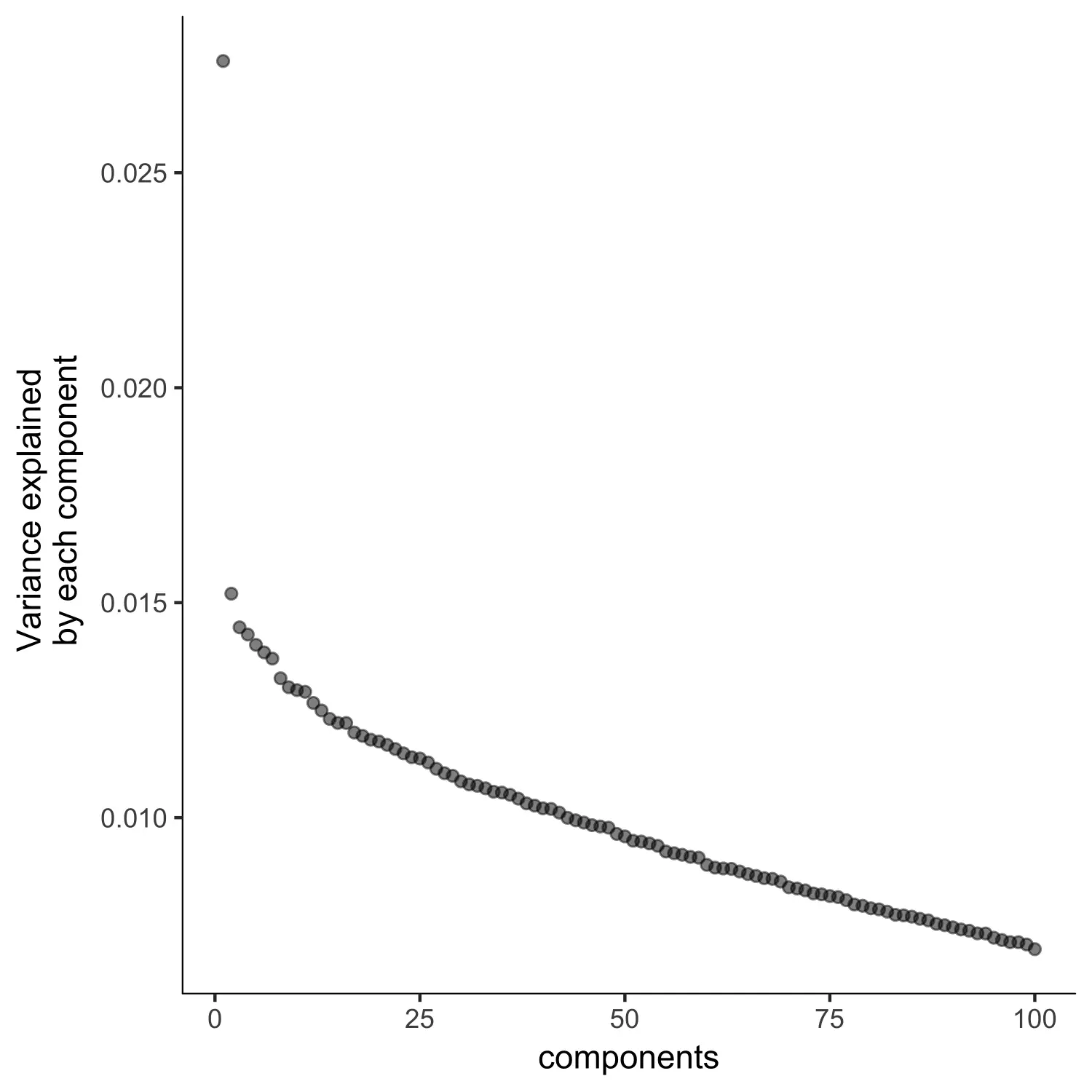
此外,我们还可以使用Monocle的dpFeature方法来选择用于数据降维的位点,dpFeature方法将会根据位点在不同细胞簇之间的差异来选择想要的位点。
plot_pc_variance_explained(agg_cds, return_all = F) #Choose 2 PCs
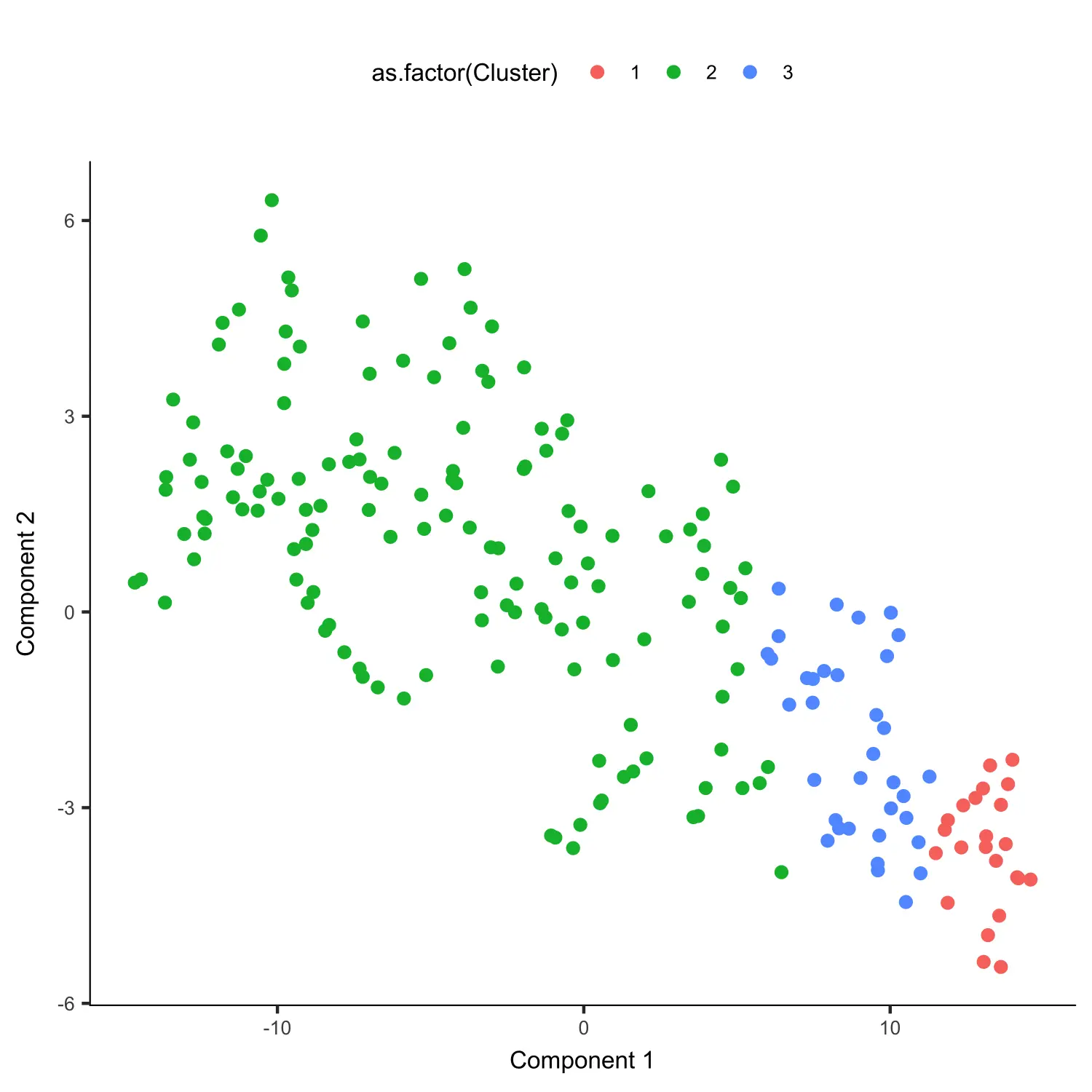
# 使用reduceDimension函数进行数据降维agg_cds <- reduceDimension(agg_cds,max_components = 2,norm_method = 'log',num_dim = 3,reduction_method = 'tSNE',verbose = T)# 使用clusterCells函数进行细胞聚类agg_cds <- clusterCells(agg_cds, verbose = F)# 聚类结果可视化plot_cell_clusters(agg_cds, color_by = 'as.factor(Cluster)')
# 根据聚类的结果对不同细胞簇之间进行差异分析clustering_DA_sites <- differentialGeneTest(agg_cds, #Takes a few minutesfullModelFormulaStr = '~Cluster')# 选择用于细胞排序的差异可及性位点ordering_sites <-row.names(clustering_DA_sites)[order(clustering_DA_sites$qval)][1:1000]
Reduce the dimensionality of the data and order cells
选择好用于细胞排序的位点后,我们需要进一步对数据进行降维,然后对降维后的结果进行细胞排序。首先,我们使用setOrderingFilter函数根据选好的位点标记筛选出用于排序的细胞。
agg_cds <- setOrderingFilter(agg_cds, ordering_sites)
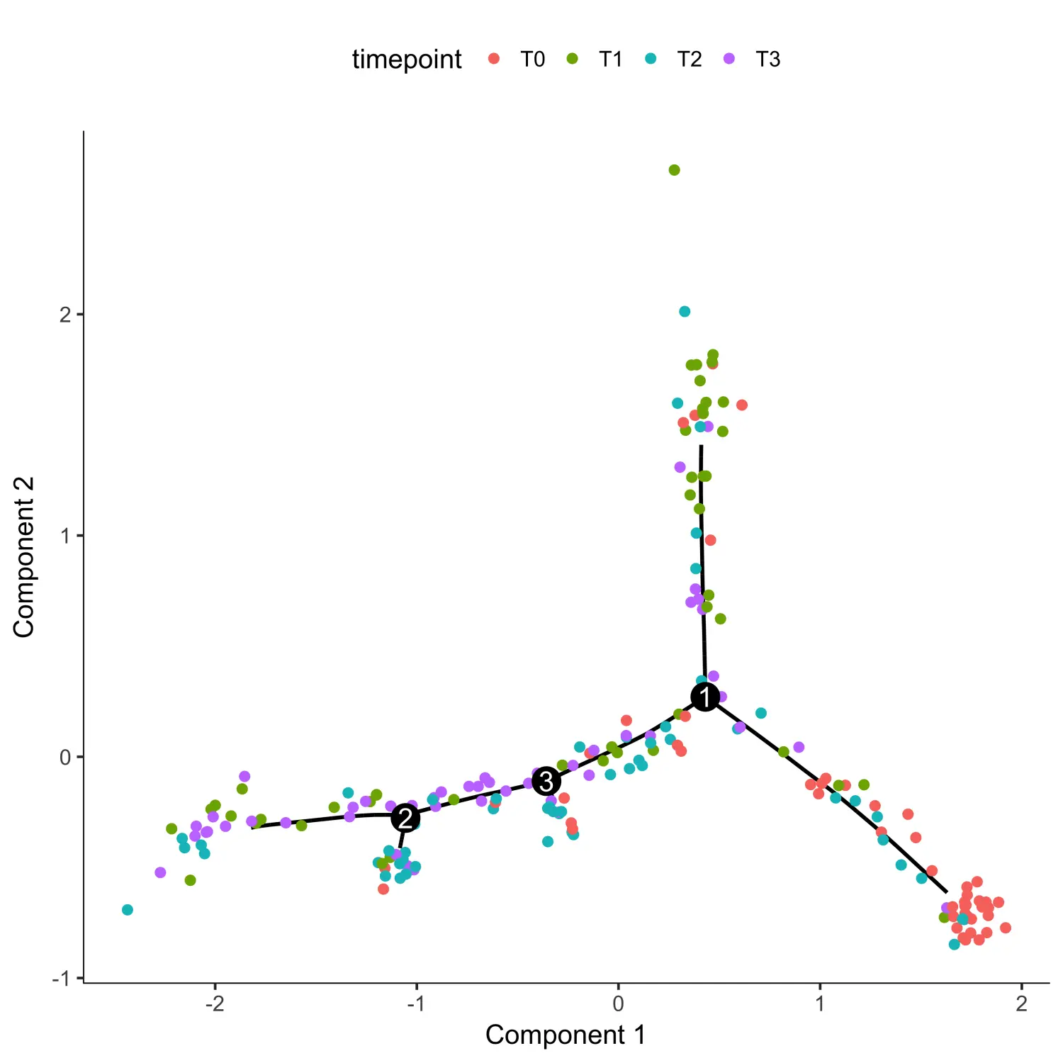
接下来,我们使用DDRTree方法对数据进行降维处理,然后对细胞进行排序构建发育轨迹。
# 使用reduceDimension函数进行数据降维agg_cds <- reduceDimension(agg_cds, max_components = 2,residualModelFormulaStr="~as.numeric(num_genes_expressed)",reduction_method = 'DDRTree')# 使用orderCells函数对降维后的结果进行细胞排序agg_cds <- orderCells(agg_cds)# 使用plot_cell_trajectory函数对细胞排序后的结果进行可视化# 根据时间点进行着色plot_cell_trajectory(agg_cds, color_by = "timepoint")
# 根据细胞状态进行着色plot_cell_trajectory(agg_cds, color_by = "State")
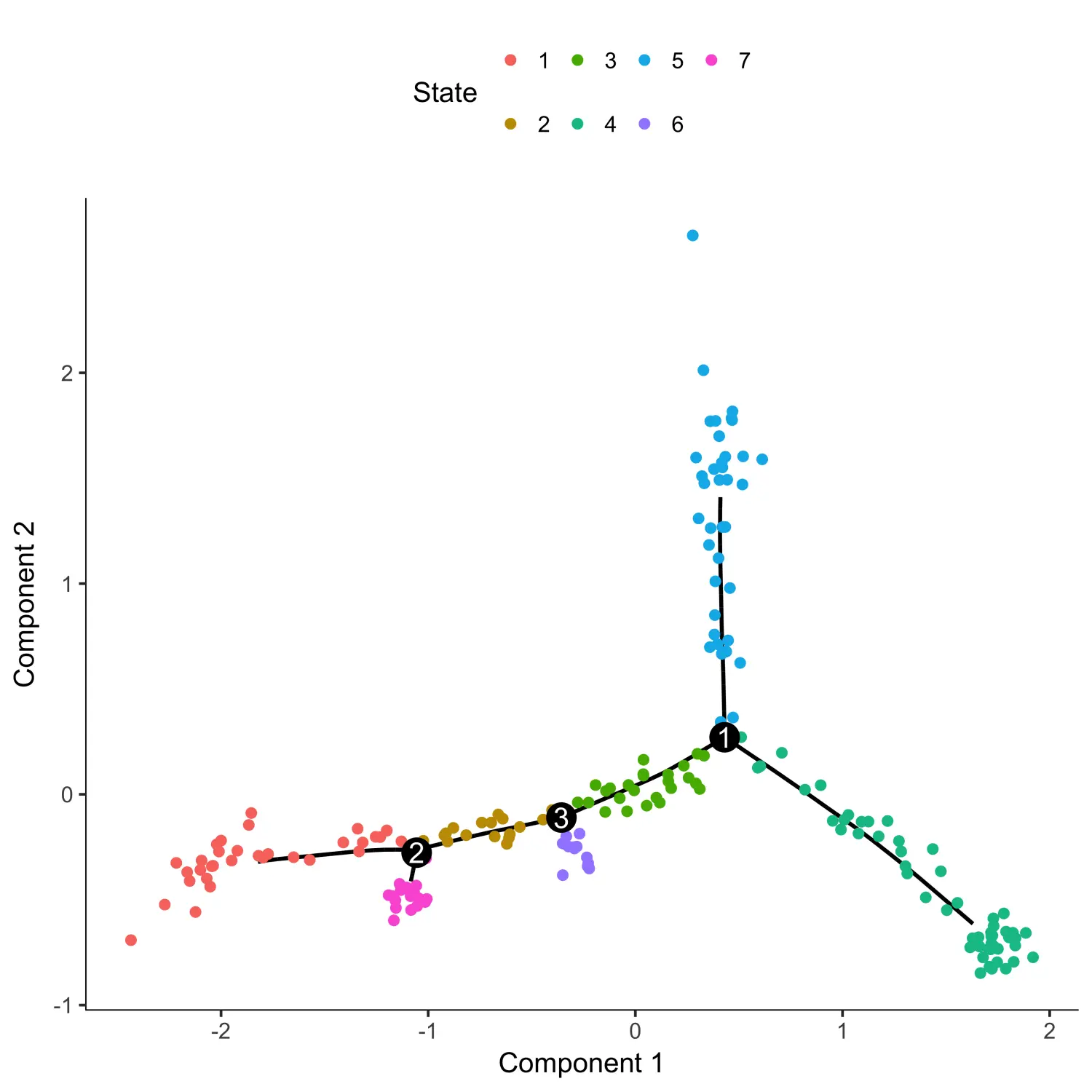
从上图中我们可以看出,伪时间应该是从state 4开始的。因此,我们可以对细胞进行重新排序,并将根状态设置为state 4。最后,可以根据伪时间对图进行着色来检查细胞排序的结果是否有意义。
agg_cds <- orderCells(agg_cds, root_state = 4)plot_cell_trajectory(agg_cds, color_by = "Pseudotime")
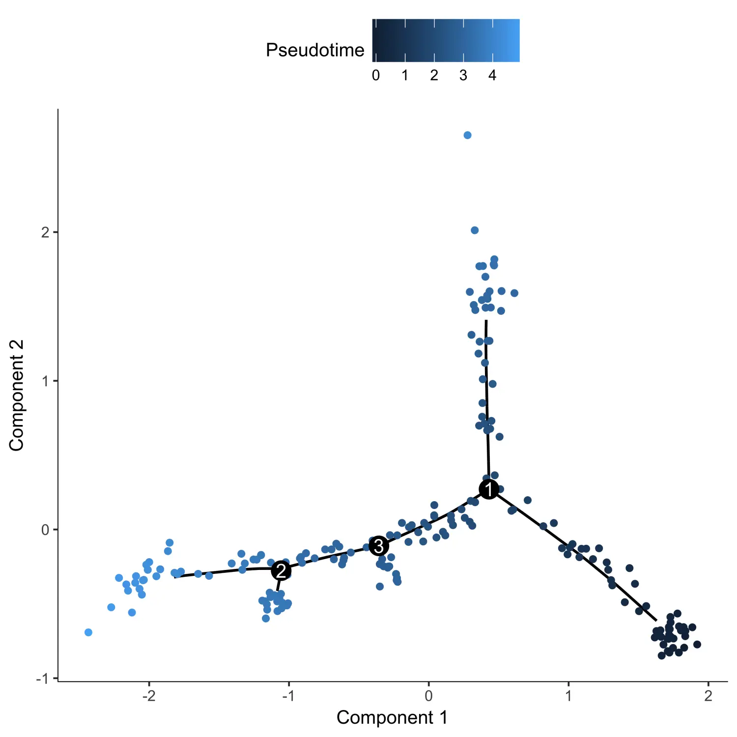
现在我们得到了每个单元所在的伪时间值,我们需要将这些伪时间值添加到原始的CDS对象中,并将细胞所处的State信息也分配回原始的CDS对象中。
pData(input_cds)$Pseudotime <- pData(agg_cds)[colnames(input_cds),]$PseudotimepData(input_cds)$State <- pData(agg_cds)[colnames(input_cds),]$State
Differential Accessibility Analysis
在我们根据伪时间分析将细胞进行排序之后,我们就可以查找基因组中染色质的可及性随伪时间变化的情况。
Visualizing accessibility across pseudotime
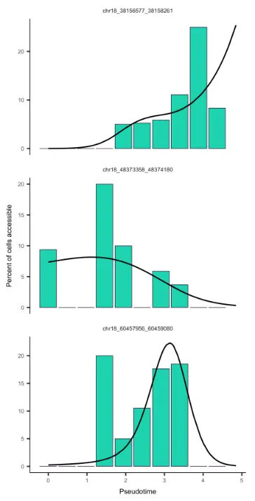
我们可以使用plot_accessibility_in_pseudotime函数可视化特定位点的染色质可及性随伪时间的变化情况。
input_cds_lin <- input_cds[,row.names(subset(pData(input_cds), State != 5))]plot_accessibility_in_pseudotime(input_cds_lin[c("chr18_38156577_38158261", "chr18_48373358_48374180", "chr18_60457956_60459080")])
Running differentialGeneTest with single cell chromatin accessibility data
在上一节中,我们使用聚合后的位点来查找cell-level级别的信息(如细胞的伪时间)。在本节中,我们将着重关注site-level级别的信息(如特定位点的染色质可及性是否随伪时间的变化而发生更改)。为此,Cicero提供了一个新的函数aggregate_by_cell_bin来实现该功能。
# 根据伪时间值将细胞分成10个类型pData(input_cds_lin)$cell_subtype <- cut(pData(input_cds_lin)$Pseudotime, 10)# 使用aggregate_by_cell_bin函数将细胞进行聚合binned_input_lin <-aggregate_by_cell_bin(input_cds_lin, "cell_subtype")
接下来,我们运行Monocle的differentialGeneTest函数来查找随伪时间变化的差异可及性位点。
diff_test_res <- differentialGeneTest(binned_input_lin,fullModelFormulaStr="~sm.ns(Pseudotime, df=3) + sm.ns(num_genes_expressed, df=3)",reducedModelFormulaStr="~sm.ns(num_genes_expressed, df=3)", cores=1)
Useful Functions
- annotate_cds_by_site
将有关peak的其他注释信息添加到CDS对象中通常是很有用的。例如,我们可能想知道哪些peak是与外显子或转录起始位点重叠的。Cicero提供了annotate_cds_by_site函数,该函数使用CDS对象和带有bed格式信息(chromosome, bp1, bp2, further columns)的数据作为输入。
head(fData(input_cds))# site_name chr bp1 bp2 num_cells_expressed# chr18_10025_10225 chr18_10025_10225 18 10025 10225 5# chr18_10603_11103 chr18_10603_11103 18 10603 11103 1# chr18_11604_13986 chr18_11604_13986 18 11604 13986 9# chr18_49557_50057 chr18_49557_50057 18 49557 50057 2# chr18_50240_50740 chr18_50240_50740 18 50240 50740 2# chr18_104385_104585 chr18_104385_104585 18 104385 104585 1feat <- data.frame(chr = c("chr18", "chr18", "chr18", "chr18"),bp1 = c(10000, 10800, 50000, 100000),bp2 = c(10700, 11000, 60000, 110000),type = c("Acetylated", "Methylated", "Acetylated", "Methylated"))head(feat)# chr bp1 bp2 type# 1 chr18 10000 10700 Acetylated# 2 chr18 10800 11000 Methylated# 3 chr18 50000 60000 Acetylated# 4 chr18 100000 110000 Methylated# 使用annotate_cds_by_site函数添加peak注释信息temp <- annotate_cds_by_site(input_cds, feat)head(fData(temp))# site_name chr bp1 bp2 num_cells_expressed overlap type# chr18_10025_10225 chr18_10025_10225 18 10025 10225 5 201 Acetylated# chr18_10603_11103 chr18_10603_11103 18 10603 11103 1 201 Methylated# chr18_11604_13986 chr18_11604_13986 18 11604 13986 9 NA <NA># chr18_49557_50057 chr18_49557_50057 18 49557 50057 2 58 Acetylated# chr18_50240_50740 chr18_50240_50740 18 50240 50740 2 501 Acetylated# chr18_104385_104585 chr18_104385_104585 18 104385 104585 1 201 Methylated
我们可以看到,使用annotate_cds_by_site函数后,peak的注释信息中添加了新的两列。overlap列表示type类所在的区间与给定peak之间重叠的碱基对的数量。如果仔细观察,我们会发现chr18_10603_11103位点实际上与feat中的两个区间之间有重叠。默认情况下,annotate_cds_by_site函数将选择最大重叠的间隔(intervals)。如果想要查看所有重叠的间隔,可以将all参数设置为TRUE。
temp <- annotate_cds_by_site(input_cds, feat, all=TRUE)head(fData(temp))# site_name chr bp1 bp2 num_cells_expressed overlap type# chr18_10025_10225 chr18_10025_10225 18 10025 10225 5 201 Acetylated# chr18_10603_11103 chr18_10603_11103 18 10603 11103 1 98,201 Acetylated,Methylated# chr18_11604_13986 chr18_11604_13986 18 11604 13986 9 NA <NA># chr18_49557_50057 chr18_49557_50057 18 49557 50057 2 58 Acetylated# chr18_50240_50740 chr18_50240_50740 18 50240 50740 2 501 Acetylated# chr18_104385_104585 chr18_104385_104585 18 104385 104585 1 201 Methylated
我们可以看到,all参数设置为TRUE后,annotate_cds_by_site函数汇报出了所有重叠的间隔。
- find_overlapping_coordinates
最后,我们可能还想知道哪些peak与基因组的特定区域发生了重叠。为此,Cicero包提供了find_overlapping_coordinates函数来实现此功能。
find_overlapping_coordinates(fData(temp)$site_name, "chr18:10,100-10,604")# [1] "chr18_10025_10225" "chr18_10603_11103"
参考来源:https://cole-trapnell-lab.github.io/cicero-release/docs/

若有收获,就点个赞吧
0 人点赞
