算法目录

前言

数据结构基本概念

1. 数据

数据是信息的载体，是描述客观事物属性的数，字符以及所有能输入到计算机中被程序识别和处理的符号合集

2. 数据元素

数据元素是数据的基本单位，通常作为一个整体进行处理。一个数据元素可由若干数据组成，数据项是构成数据元素不可分割的最小单位。例如，学生档案是一个数据元素，它是由学号，性别，名字等数据项组成的。

3. 数据对象

数据对象是具有相同数据元素的合集。是一个数据的子集。例如， 整数的数据对象是N={0，±1，±2，。。。}

4. 数据类型

1. 原子类型：其值不可再分的数据类型

2. 结构类型： 其值可以在分解为若干分量

3. 抽象数据类型：抽象数据与之相关的操作

5. 抽象数据结构

抽象数据类型（ADT）是指一个数学模型及其定义在该模型的一系列操作。通常用数据对象，数据关系，基本操作集三元组来表示抽象数据类型。

6. 数据结构

数据之间存在相互的关系，这种关系就称为数据结构。数据机构包括三方面：逻辑结构，储存结构，数据的运算

数据结构三要素

1. 数据的逻辑结构

2. 数据的储存结构

3. 数据的运算

算法基本概念与度量

1. 基本概念

算法（Algorithm）是对特定问题求最优解的一种描述，一个算法需要具备5个重要特征：

1. )有穷性。对于任何合法的输入值必须在有穷步以后结束，且每一步再有穷时间内完成
2. ）确定性。 保证不会出现薛定谔的量子不确定状态，即同样条件下的同一输入值得出不同的结果
3. ）可行性。算法描述中的操作是可以做到的，可用induction归纳法证明出来
4. ）输入。一个算法有零个或者多个输入，来自于某个特定的对象的合集
5. ）输出。一个算法有一个或多个输出，输出与输入有特定关系的量。

2. 时间复杂度

一行指令被重复的频次就是频度。Σni=1频度=T(n)
算法中的基本运算频度是f(n)，算法的时间复杂度记为T(n)=O(f(n)).

Asymptotic Analysis——渐近分析

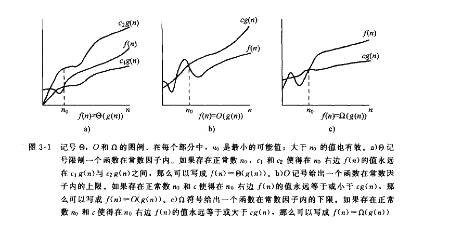
big 0 notation 三个rules

1. ignore constant factor
2. Combine fixed number of terms with same complexity（special case： n terms）

3. consider only the most higher dimension power

   3. 空间复杂度

   一个算法所耗费的储存空间。
   记为S(n)=O(g(n))

4. 空间复杂度 O(1)

   int i = 1;
   int j = 2;
   i++ ;
   ++j;
   //代码中的 i、j 所分配的空间都不随着处理数据量变化，因此它的空间复杂度 S(n) = O(1)

5. 空间复杂度 O(n) ```python a = n x = [None]*a print(x)

   [None, None, None, None, None, None, None, None, None, None，。。。。]

   创建了n个空间，所以占用了这么多的空间，即 S(n) = O(n)

常见的复杂度不多，从低到高排列就这么几个: O(1) 、 O(log(n)) 、 O(n) 、 O(n2)
---
<a name="L1QLs"></a>
# 线性表
<a name="KKc2E"></a>
## 数组
<a name="k42Tp"></a>
## 链表
---
<a name="x2QQ4"></a>
# 散列表
---
<a name="C8hUj"></a>
# 树
---
<a name="EMw87"></a>
# 图
---
<a name="VjIC4"></a>
# 复杂度分析
---
<a name="y8JxZ"></a>
# 基本算法思路
---
<a name="YMbqw"></a>
# 排序
---
<a name="Sy28m"></a>
# 搜索
---
<a name="gbybK"></a>
# 查找
---
<a name="E1FG1"></a>
# 字符串匹配
---
<a name="w0ByP"></a>
# 不精确一维搜索-Armijo-Goldstein准则与Wolfe-Powell准则（ama505）
不精确一维搜索就是在区间【0，∞）上求近似最小值，用一个可以接受的参数来表示这个近似值，使用条件是函数 f ′ ( 0 ) < 0。<br />主要有两种方法：Armijo-Goldstein法和Wolfe-Powell法
**Armijo-Goldstein准则：**<br />两个核心思想，1. 目标函数有足够的下降 2. 一维搜索的步长λ不应该太小。<br />每一次下降的步长够小才能保证近似值的精准度，就像牛顿法那样分的步骤越多越精准，但是步长太小也会导致你的机器学习一直在在地停留没有进步。
数学表达式：<br />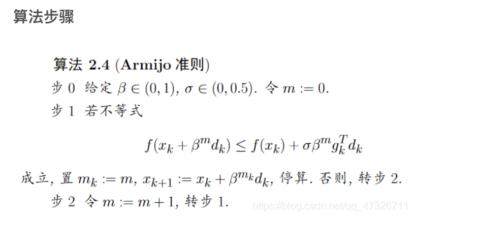![](https://cdn.nlark.com/yuque/__latex/103629657e6e572e26a5b583692bc98c.svg#card=math&code=%5C%5C%5C%5C%5C%0Af%28x%20%0Ak%0A%20%2B%CE%BB%20%0Ak%0A%E2%80%8B%0A%20d%20%0Ak%0A%20%29%E2%88%92f%28x%20%0Ak%0A%20%29%E2%89%A4%CE%BB%20%0Ak%0A%E2%80%8B%0A%20%CF%81g%20%0Ak%0AT%0A%E2%80%8B%0A%20d%20%0Ak%0A%20%0A%E2%80%8B%0A%EF%BC%881%EF%BC%89%0A&id=Rd0OH)
![](https://cdn.nlark.com/yuque/__latex/f729467b3eb6ab46333969fa75487180.svg#card=math&code=f%28x%20%0Ak%0A%20%2B%CE%BB%20%0Ak%0A%E2%80%8B%0A%20d%20%0Ak%0A%20%29%E2%88%92f%28x%20%0Ak%0A%20%29%E2%89%A5%CE%BB%20%0Ak%0A%E2%80%8B%0A%20%281%E2%88%92%CF%81%29g%20%0Ak%0AT%0A%E2%80%8B%0A%20d%20%0Ak%0A%5C%20%20%20%0A%E2%80%8B%282%29%0A%5C%5C%0A%0A%E5%85%B6%E4%B8%AD%EF%BC%8C0%20%3C%20%CF%81%20%3C%20%0A1%2F2&id=lUL98)
![image.png](https://cdn.nlark.com/yuque/0/2021/png/22418899/1632496722557-da9b7450-1d14-4934-b2c7-dbeee50ee184.png#clientId=u1f4171d7-899e-4&crop=0&crop=0&crop=1&crop=1&from=paste&height=378&id=u1576a0af&margin=%5Bobject%20Object%5D&name=image.png&originHeight=484&originWidth=939&originalType=binary&ratio=1&rotation=0&showTitle=false&size=109787&status=done&style=none&taskId=u32f7ba21-3445-401b-ad70-fc5820dce4b&title=&width=733.5)<br />Matlab实现
```matlab
function mk=armijo(xk,dk )
beta=0.5;  sigma=0.2;
m=0; mmax=20;
while (m<=mmax)
    if(fun(xk+beta^m*dk)<=fun(xk)+sigma*beta^m*gfun(xk)'*dk)
        mk=m;  break;
    end
    m=m+1;
end
alpha=beta^mk
newxk=xk+alpha*dk
fk=fun(xk)
newfk=fun(newxk)
————————————————
版权声明：本文为CSDN博主「斑马L*」的原创文章，遵循CC 4.0 BY-SA版权协议，转载请附上原文出处链接及本声明。
原文链接：https://blog.csdn.net/qq_47326711/article/details/118075514

python实现

def armijo_goldstein(f,df,d,x,lambda_max,p,t):
    '''
    f=函数
    df=导数
    d= 矢量方向
    x=当前点
    lambda_max=最大步长
    p= 公示里面的p用来调整步长的
    t= 上一步的时间相当于游戏存档
    '''
    true_false = 0
    a= 0
    b = lambda_max
    fx = f(x)
    df = df(x)
    last_step = fx
    next_step = np.dot(df,d) '用numpy朝着d方向精确求导一个梯度'
    lambda0 = b*random.unifrom(0,1)
    while(true_false==0):
        new_fx = f(x+lambda0 * d)
        curr_step = new_fx
        if (curr_step-last_step) <= (p * lambda0 * next_step): '如果近似步长小于最大上界'
            if (curr_step - last_step) >= ((1-p) * lambda0 * next_step): '近似步长大于最小下界'
                true_false = 1
            else:
                '步长太小，使用binary提高a来寻找更适中的lambda'
                a = lambda0
                b = b
                if (b < lambda_max):
                    lambda0 = (a+b)/2
                else: '梯度爆炸问题，回到上一步存档'
                    lambda0 = t* lambd0 
        else:'过大了，减少上界重新选步长'
            a = a
            b = lambda0
            lambda0 = (a+b) /2
     return   lambda0      
  '''
   版权声明：蒙特卡洛树正在找图灵的猫
   '''

Wolfe-Powell准则（ama505）

Armijo-Goldstein准则可能会把极小值点（可接受的区间）判断在外，因此使用wolfe-powell准则
wolfe-powell准则也有两个数学表达式，第一个和armijo-goldstein一样，第二个是：

这个是一个关于梯度的式子。

算法：
【1】筛选数据
在搜索区间[0,_λ_max] 上选定初始探测点λ0，代入计算好的 f ( 0 ) , f ′ ( 0 ) ，给出可接受系数

【2】检查步长lambda合格否
如果，成功，取下一步，否则缩小上界重新选择下探点
【3】检查下探点是否过小
步骤类似于python实现
[

](https://blog.csdn.net/qq_43940950/article/details/117566544)

拟牛顿法BFGS（ama505）

1. 什么是拟牛顿法

牛顿法可以快速收敛，迭代次数少但是每一次都需要计算矩阵的逆导致计算量很大。因此拟牛顿法就是引入了Hessian矩阵的近似矩阵可以避免每次迭代都计算矩阵的逆。它的收敛速度介于梯度下降法和牛顿法之间。

1. 原理

在机器学习中经常碰到非线性优化问题，一些算法试图求解一个非线性极小点，最常用的就是BFGS和L-BFGS算法。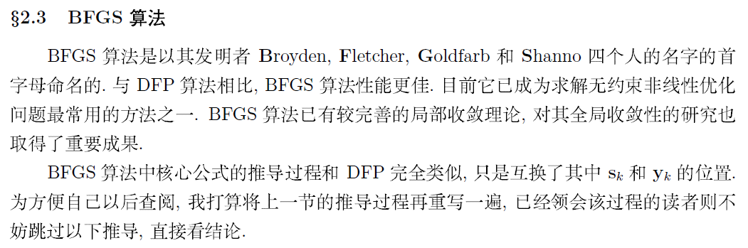

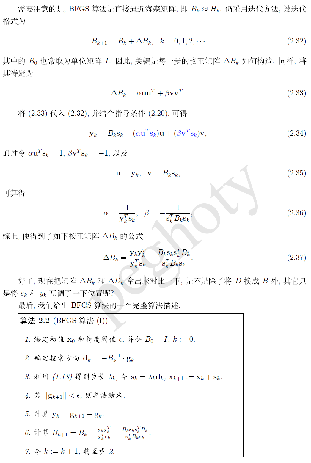
1. 实现

其实现在python里面有scipy包里面的optimizer内置函数可以直接用，已经有更好的optimizer了，比如SGD/BGD

#coding:UTF-8  
from numpy import *  
from function import *  
def bfgs(fun, gfun, x0):  
    result = []  
    maxk = 500  
    rho = 0.55  
    sigma = 0.4  
    m = shape(x0)[0]  
    Bk = eye(m)  
    k = 0  
    while (k < maxk):  
        gk = mat(gfun(x0))#计算梯度  
        dk = mat(-linalg.solve(Bk, gk))  
        m = 0  
        mk = 0  
        while (m < 20):  
            newf = fun(x0 + rho ** m * dk)  
            oldf = fun(x0)  
            if (newf < oldf + sigma * (rho ** m) * (gk.T * dk)[0,0]):  
                mk = m  
                break  
            m = m + 1  
        #BFGS校正  
        x = x0 + rho ** mk * dk  
        sk = x - x0  
        yk = gfun(x) - gk  
        if (yk.T * sk > 0):  
            Bk = Bk - (Bk * sk * sk.T * Bk) / (sk.T * Bk * sk) + (yk * yk.T) / (yk.T * sk)  
        k = k + 1  
        x0 = x  
        result.append(fun(x0))  
    return result  
'''
代码来源：https://blog.csdn.net/xiaopihaierletian/article/details/73950484
'''

共轭梯度法(Conjugate Gradient Method)（ama505）

1. 介绍

共轭梯度法（Conjugate Gradient）是介于最速下降法与牛顿法之间的一个方法，它仅需利用一阶导数信息，但克服了最速下降法收敛慢的缺点，又避免了牛顿法需要存储和计算Hesse矩阵并求逆的缺点，共轭梯度法不仅是解决大型线性方程组最有用的方法之一，也是解大型非线性最优化最有效的算法之一。 在各种优化算法中，共轭梯度法是非常重要的一种。其优点是所需存储量小，具有步收敛性，稳定性高，而且不需要任何外来参数。
共轭梯度法最初由Hesteness和Stiefel于1952年为求解线性方程组而提出的。后来，人们把这种方法用于求解无约束最优化问题，使之成为一种重要的最优化方法。
共轭梯度法的基本思想是把共轭性与最速下降方法相结合，利用已知点处的梯度构造一组共轭方向，并沿这组方向进行搜素，求出目标函数的极小点。根据共轭方向基本性质，这种方法具有二次终止性。

1. 原理与数学推理

https://www.cnblogs.com/walccott/p/4956966.html
https://blog.csdn.net/Liang_Ling/article/details/78552788

1. 实现

共轭梯度法。一种求解数学特定线性方程组Ax=b的数值解的迭代方法。
要求矩阵A对称（symmetric）且正定（positive definite）。

def Conjugate_Gradient(e=1e-1, lambda0=0.01,x_init):
    x = x_init
    df = grad(x)'grad求导‘
    p = -df
    costs = [cost(x)]
    while abs(df[0]) > e or abs(df[1]) > e:   
        x1 = armijo_goldstein(x,df,p,lamda0) '一维搜索都可以用‘
        df1 = grad(x1)
        alpha_t = alpha(df1, df)    '计算两次求导梯度差‘
        p1 = -df1 + alpha_t*p
        current_cost = cost(x1)        '用新的x1算出新的cost‘
        costs.append(current_cost)
        '更新参数‘
        x = x1
        df = df1
        p = p1
    return costs, x
  '''
  蒙特卡洛树正在找图灵的猫
  ‘’‘

深度学习入门

环境安装

#环境安装
#python
#https://www.python.org/downloads/
GPU>= 1080ti
RAM >= 64gb
方法二：
使用google colaboratory
方法三：
使用Jupyter Notebook
下载CUDA/Anaconda
https：//oreil.ly/9hAxg
安装pytorch
conda install pytorch torchvision -c pytorch 
jupyter notebook
import torch
print(torch.cuda.is_available())

#导入numpy
import numpy as np
x = np.array([1,2,3])
y = np.array([2,4,6])
# >>>x + y = ([3,6,9])
#matrix muultiplication
x = ([[1,2],[3,4]])
y = ([10,20])
# >>>x*y = ([[10,40],[30,80]])
#转化为一维数组
x = x.flatten()
import matplotlib.pyplot as plt
#draw graph
plt.plot(x,y1, label = "sales")
plt.plot(x,y2,linestyle='--',label = "cost")
plt.xlabel("x")
plt.ylabel("y")
plt.title("sales & cost")
img = imread('../Destop/lena.png')
plt.show()
#与门
def and_door(x1,x2):
  x = np.array([x1,x2])
  w = np.array([0.5,0.5])
  theta = -0.8
  tmp = np.sum(w*x)+theta
  if tmp <= 0 :
    return 0
  else:
    return 1
#与非门
def NAND(x1,x2):
  x = np.array([x1,x2])
  w = np.array([-0.5,-0.5])
  theta = 0.8
  tmp = np.sum(w*x)+theta
  if tmp <= 0 :
    return 0
  else:
    return 1
#或门
def or_door(x1,x2):
  x = np.array([x1,x2])
  w = np.array([0.5,0.5])
  theta = -0.3
  tmp = np.sum(w*x)+theta
  if tmp <= 0 :
    return 0
  else:
    return 1
#异或门
def XOR(x1,x2):
  s1 = NAND(x1,x2)
  s2 = or_door(x1,x2)
  y = and_door(s1,s2)
  return y

非线性函数activation function

#activation function
#非线性函数
#sigmoid fun
#h(x) = 1/(1+exp(-x))
def sigmoid(x):
  return 1/(1 + np.exp(-x))
#step function
def step_fun(x):
  y = x >0
  return y.astype(np.int)

线性函数

#ReLU
def relu(x):
    return np.maximum(0,x)

多维数组

A= np.array([1,2,3,4])
B = np.array([[1,2],[3,4],[5,6]])
np.ndim(A) = 1
np.ndim(B) = 2
A.shape = (4,)
B.shape = (3,2)
A.shape[0] = 4
#shape is tuple 
#mult
np.dot(A,B)

基本三元神经实现

def network():
    net = {}
    net['w1'] = np.array([ [x1,x2,x3],[y1,y2,y3] ])
    net['w2'] = np.array([ [x1,x2],[y1,y2],[z1,z2] ])
    net['w3'] = np.array([  [x1,x2,x3],[y1,y2,y3] ])
    net['b1'] = np.array([  [t1,t2,t3] ])
    net['b2'] = np.array([  [t1,t2] ])
    net['b3'] = np.array([  [t1,t2] ])
    return net
def forward(net,x):
    w1,w2,w3 = net['w1'], net['w2'], net['w3']
    b1,b2,b3 = net['b1'], net['b2'], net['b3']
    a1 = np.dot(x,w1) +b1
    z1 = sigmoid(a1)
    a2 = np.dot(z1,w2) +b2
    z2 = sigmoid(a2)
    a3 = np.dot(z2,w3) + b3
    res = identity_function(a3)  #let output.shape = input.shape
    return res
net = network()
x = np.array([1,0.5])
y = forward(net,x)

很多事情，尽量更新

softmax函数

softmax是一个总是输出0到1之间的实数的一个函数，其实可以理解把每一个结果变成一个可能发生的概率。因为即使使用了softmax各个元素之间的大小关系也不会发生变化。

def softmax(a):
    exp_a = np.exp(a)
    sum_exp_a = np.sum(exp_a)
    res = exp_a / sum_exp_a
    return res 
#因为计算机的运算存在缺陷会导致指数函数的值变得非常大没办法计算因此直接使用：
def softmax(x):
    if x.ndim == 2:
        x = x.T
        x = x - np.max(x, axis=1) #稳定概率，剪掉最大的元素，axis=0是列，axis=1是行
        y = np.exp(x) / np.sum(np.exp(x), axis=0)
        return y.T 
    x = x - np.max(x) # 溢出对策
    return np.exp(x) / np.sum(np.exp(x))

MNIST 数据集

mnist数据集就是一堆从0到9的手写数字图像集：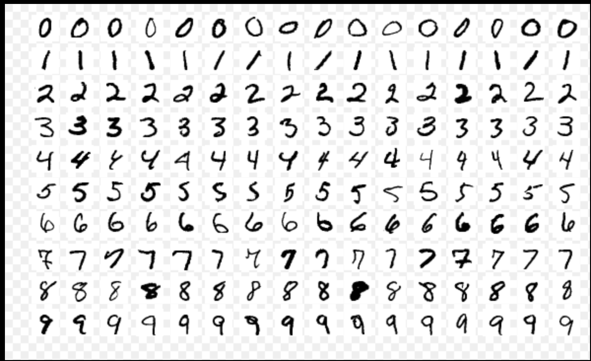

使用这个mnist.py可以将数据集下载并转化成Numpy数组来处理

# coding: utf-8
try:
    import urllib.request
except ImportError:
    raise ImportError('You should use Python3')
import os.path
import gzip
import pickle
import os
import numpy as np
url_base = 'http://yann.lecun.com/exdb/mnist/'
key_file = {
    'train_img':'train-images-idx3-ubyte.gz',
    'train_label':'train-labels-idx1-ubyte.gz',
    'test_img':'t10k-images-idx3-ubyte.gz',
    'test_label':'t10k-labels-idx1-ubyte.gz'
}
dataset_dir = os.path.dirname(os.path.abspath(__file__))
save_file = dataset_dir + "/mnist.pkl"
train_num = 60000
test_num = 10000
img_dim = (1, 28, 28)
img_size = 784
def _download(file_name):
    file_path = dataset_dir + "/" + file_name
    if os.path.exists(file_path):
        return
    print("Downloading " + file_name + " ... ")
    urllib.request.urlretrieve(url_base + file_name, file_path)
    print("Done")
def download_mnist():
    for v in key_file.values():
       _download(v)
def _load_label(file_name):
    file_path = dataset_dir + "/" + file_name
    print("Converting " + file_name + " to NumPy Array ...")
    with gzip.open(file_path, 'rb') as f:
            labels = np.frombuffer(f.read(), np.uint8, offset=8)
    print("Done")
    return labels
def _load_img(file_name):
    file_path = dataset_dir + "/" + file_name
    print("Converting " + file_name + " to NumPy Array ...")    
    with gzip.open(file_path, 'rb') as f:
            data = np.frombuffer(f.read(), np.uint8, offset=16)
    data = data.reshape(-1, img_size)
    print("Done")
    return data
def _convert_numpy():
    dataset = {}
    dataset['train_img'] =  _load_img(key_file['train_img'])
    dataset['train_label'] = _load_label(key_file['train_label'])    
    dataset['test_img'] = _load_img(key_file['test_img'])
    dataset['test_label'] = _load_label(key_file['test_label'])
    return dataset
def init_mnist():
    download_mnist()
    dataset = _convert_numpy()
    print("Creating pickle file ...")
    with open(save_file, 'wb') as f:
        pickle.dump(dataset, f, -1)
    print("Done!")
def _change_one_hot_label(X):
    T = np.zeros((X.size, 10))
    for idx, row in enumerate(T):
        row[X[idx]] = 1
    return T
def load_mnist(normalize=True, flatten=True, one_hot_label=False):
    """读入MNIST数据集
    Parameters
    ----------
    normalize : 将图像的像素值正规化为0.0~1.0
    one_hot_label : 
        one_hot_label为True的情况下，标签作为one-hot数组返回
        one-hot数组是指[0,0,1,0,0,0,0,0,0,0]这样的数组
    flatten : 是否将图像展开为一维数组
    Returns
    -------
    (训练图像, 训练标签), (测试图像, 测试标签)
    """
    if not os.path.exists(save_file):
        init_mnist()
    with open(save_file, 'rb') as f:
        dataset = pickle.load(f)
    if normalize:
        for key in ('train_img', 'test_img'):
            dataset[key] = dataset[key].astype(np.float32)
            dataset[key] /= 255.0
    if one_hot_label:
        dataset['train_label'] = _change_one_hot_label(dataset['train_label'])
        dataset['test_label'] = _change_one_hot_label(dataset['test_label'])
    if not flatten:
         for key in ('train_img', 'test_img'):
            dataset[key] = dataset[key].reshape(-1, 1, 28, 28)
    return (dataset['train_img'], dataset['train_label']), (dataset['test_img'], dataset['test_label']) 
if __name__ == '__main__':
    init_mnist()

#接着可以使用load_mnist()读入mnist数据
#normalize设置是否将图像正规化为0～1的实数，否则像素保持0～255
#flatten设置是否展开图像为一维，否则保持1*28*28
#one-hot表示仅仅正确的解的标签为1其余标签为0
# coding: utf-8
import sys, os
sys.path.append(os.pardir)  # 为了导入父目录的文件而进行的设定
import numpy as np
from dataset.mnist import load_mnist
from PIL import Image
def img_show(img):
    pil_img = Image.fromarray(np.uint8(img))
    pil_img.show()
(x_train, t_train), (x_test, t_test) = load_mnist(flatten=True, normalize=False)
img = x_train[0]
label = t_train[0]
print(x_train.shape) #60000,784
print(t_train.shape) #60000
print(x_test.shape) #10000,784
print(t_test.shape) #10000
print(label)  # 5
print(img.shape)  # (784,)
img = img.reshape(28, 28)  # 把图像的形状变为原来的尺寸
print(img.shape)  # (28, 28)
img_show(img)

#接着使用之前的sigmoid，softmax和forward来进行基本的机器学习
# coding: utf-8
import sys, os
sys.path.append(os.pardir)  # 为了导入父目录的文件而进行的设定
import numpy as np
import pickle
from dataset.mnist import load_mnist
def softmax(x):
    if x.ndim == 2:
        x = x.T
        x = x - np.max(x, axis=0)
        y = np.exp(x) / np.sum(np.exp(x), axis=1)
        return y.T 
    x = x - np.max(x) # 溢出对策
    return np.exp(x) / np.sum(np.exp(x))
def sigmoid(x):
    return 1 / (1 + np.exp(-x))
def get_data():
    (x_train, t_train), (x_test, t_test) = load_mnist(normalize=True, flatten=True, one_hot_label=False)
    return x_test, t_test
def init_network():
    with open("sample_weight.pkl", 'rb') as f:
        network = pickle.load(f)
    return network
def predict(network, x):
    W1, W2, W3 = network['W1'], network['W2'], network['W3']
    b1, b2, b3 = network['b1'], network['b2'], network['b3']
    a1 = np.dot(x, W1) + b1
    z1 = sigmoid(a1)
    a2 = np.dot(z1, W2) + b2
    z2 = sigmoid(a2)
    a3 = np.dot(z2, W3) + b3
    y = softmax(a3)
    return y
x, t = get_data()
network = init_network()
accuracy_cnt = 0
for i in range(len(x)):
    y = predict(network, x[i])
    p= np.argmax(y) # 获取概率最高的元素的索引
    if p == t[i]:
        accuracy_cnt += 1
print("Accuracy:" + str(float(accuracy_cnt) / len(x)))
##Accuracy:0.9352

批处理batch

例如输入数据是100x784，然后输出数据是100x10.这种打包数据是batch，批处理可以缩短每张图像处理的时间

#批处理的实现·
x, t  = get_data()
network = init_network()
batch_size = 100
acc = 0
for i in range(0,len(x),batch_size):
    x_batch = x[i:i+batch_size]
    y_batch = predict(network,x_batch)
    p = np.argmax(y_batch,axis = 1)
    #p == t[i:i+batch_size] 是布尔值，将np.sum会将所有的TRUE加起来
    acc += np.sum(p == t[i:i+batch_size])
print("Accuracy:" + str(float(acc)/len(x)))

#argmax
a = array([[10, 11, 12],
           [13, 14, 15]])
np.argmax(a)
>>5
np.argmax(a, axis=0)#axis=0 从列出发
>>array([1, 1, 1])
np.argmax(a, axis=1)#从行出发
>>array([2, 2])

训练与测试数据

在计算机视觉领域中，常用的特征量为SIFT，SURF，HOG，然后使用这个特征量将图像数据转化为向量。
对转化后的向量使用机器学习的SVM，KNN等分类器进行学习。
在机器学习中，一般将数据分为训练数据和测试数据。有训练数据的机器学习也称为监督学习，反之为无监督学习。某个数据过度拟合就是过拟合over fitting

损失函数