- Kaggle房价预测比赛,使用统计学方法进行数据分析与处理例如target encoding和PCA,然后基于XgBoost建立模型进行预测
- 人脸考勤打卡系统
- 基于RNN和LSTM的英文垃圾邮件分类系统
- 基于用户的英文评论的药品评级推荐系统
- https://www.kaggle.com/aashita/word-clouds-of-various-shapes">reference: https://www.kaggle.com/aashita/word-clouds-of-various-shapes
- importing libraries
- importing libraries for Deep Learning
- connect to google drive
- transfer images intp array of numbers
- https://keras.io/api/preprocessing/image/">references: https://keras.io/api/preprocessing/image/
- since our data are label into 2 folders cats and dogs, wo we choice use
- data_generator.flow_from_directory that can directly read data in two floders
- 4. training训练
Kaggle房价预测比赛,使用统计学方法进行数据分析与处理例如target encoding和PCA,然后基于XgBoost建立模型进行预测
1. 数据集介绍
数据集是波士顿出售中的房子的信息,训练数据集总共1460条数据,包括79个可预测房价的变量,和一个房价变量.
测试集有1459条数据,除了没有房价其他变量类型一样有79种. 变量很多包括建筑类型,街道,房屋面积,楼层,地下室,游泳池,浴室和车库质量与数量,甚至于屋顶材料等等,因此很多变量是string字符串并不能直接用来训练.
2. imputation清洗数据
我决定采用的模型是基于决策树decision tree 的XGboost,
通过研究数据我们发现变量LotFrontage和最终的房价strong correlated 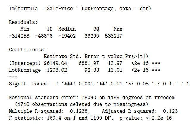
但是它有很多空数据,所以我们需要补上空数据
首先我们做一个imputation.也就是通过一些统计学的方法将合理的数据替换一些遗失的空数据.
用其中LotArea这个变量通过求最大似然数可以求得LotFrontage的近似数以填补missing data.
3. target encoding
由于数据中很多数据并不是数字而是string字符串,我们需要转换为数字才可以利用为训练特征.
用类别对应的标签的期望来代替原始的类别,所谓的期望,简单理解为均值即可。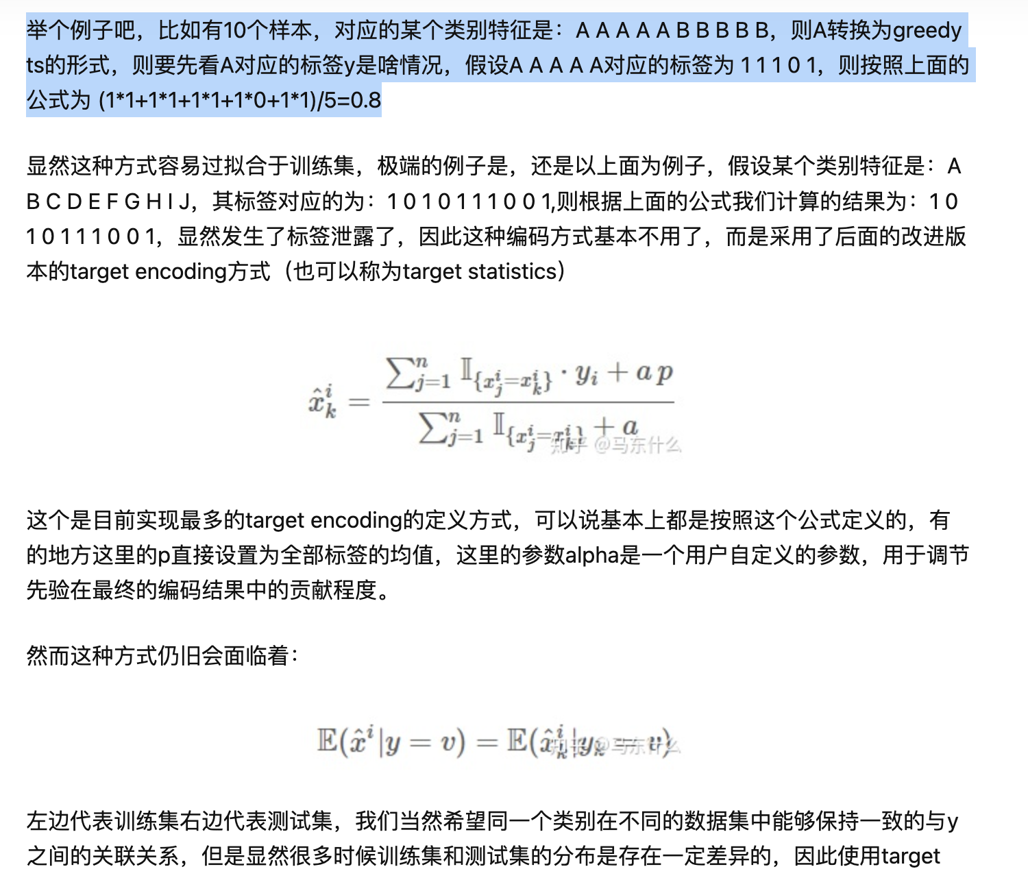
target encoding可以理解成一种类似于one-hot类标签方法,会有一定的偏差.
3. 主成分分析PCA
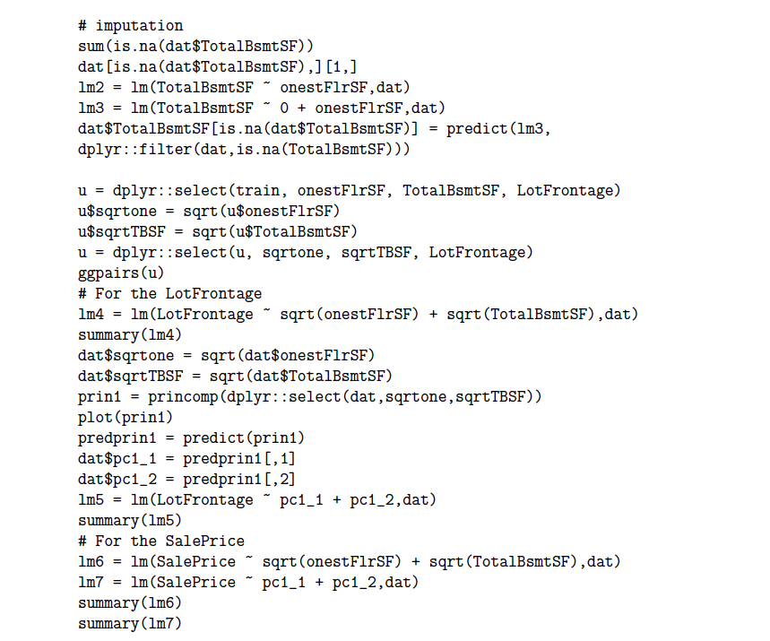
由于数据量大过于复杂会有很多的noise噪音导致结果失去正态分布产生较大偏差,因为我们需要将一些噪音去掉,将所有需要的训练数据组合成一个大的矩阵,使用主成分分析降纬去掉噪音,精简训练数据.
4. 搭建模型基于决策树的XgBoost
XGBoost(eXtreme Gradient Boosting)极致梯度提升,是基于GBDT的一种算法。(Gradient Boosting Decision Tree,GBDT),他们都是是一种基于boosting集成思想的加法模型,训练时采用前向分布算法进行贪婪的学习,每次迭代都学习一棵CART树来拟合之前 t-1 棵树的预测结果与训练样本真实值的残差。
2016年,陈天奇在论文《 XGBoost:A Scalable Tree Boosting System》中正式提出。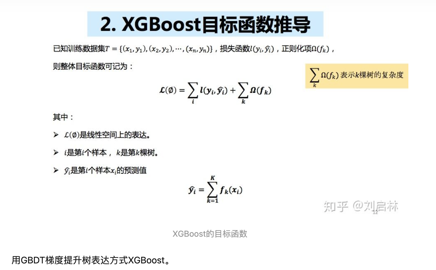
1.二阶泰勒展开,去除常数项

2. 正则化项展开,去除常数项

3. 合并一次项系数,二次项系数

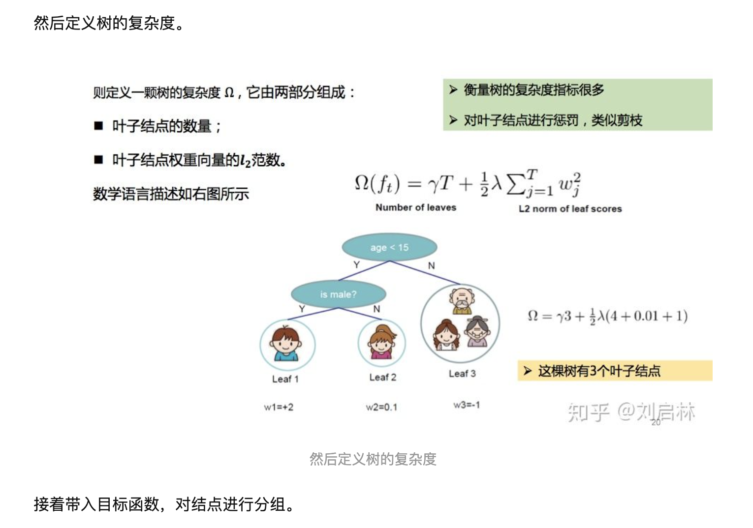
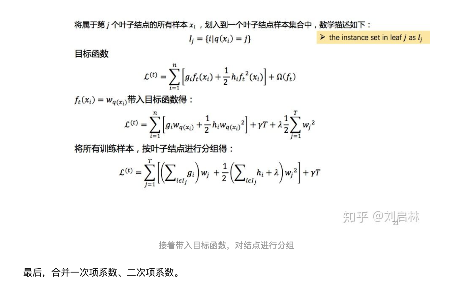
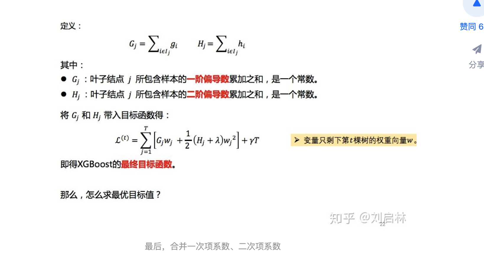

目标值最小则是目标函数最小解
以下是R语言代码实现: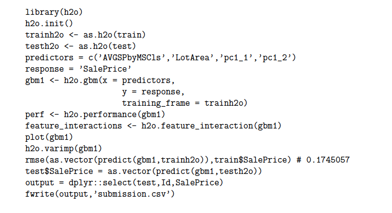

- 均方根误差RMSE:计算平方和的根,测量预测向量与目标值向量之间的距离,又称为欧几里得范数,L2范数
- 平均绝对误差MAE:计算绝对值的总和,对应于L1范数,又称为曼哈顿距离
人脸考勤打卡系统
1. 介绍
首先录入人脸信息,接着切换识别模式,扫描人脸打卡
use python demo_full.py --{variable}={value}-h, --help show this help message and exit--mode MODE mode:reg,recog -> input face information、face recognition--id ID face ID,int, not repeated--name NAME English people name--interval INTERVAL register face intyerval per second--count COUNT register how many picture of your--w W windows width,default 1/2 of computer windows--h H height width,default 1/2 of computer windows--detector DETECTOR choice detector,option: haar、hog、cnn--threshold THRESHOLD from 1- 0, more low value means more recognition points so that more clear--record RECORD detect whether video is recorded#录入人脸#python demo_full.py --mode=reg --id={face_ID,int} --name={your_name} --interval={int, per second} --count={int, how many picture} --w={int} --h={int}python demo_full.py --mode=reg --id=1 --name='yourname' --interval=5 --count=10#人脸识别#python demo_full.py --mode=recog --detector={choice detector,option: haar、hog、cnn} --threshold={number from 0-1 } --record={bool}python demo_full.py --mode=recog --detector=haar --threshold=0.2 --record=True
2. 模型搭建
"""人脸考勤系统(可以运行在CPU)1、人脸检测:2、注册人脸,将人脸特征存储进feature.csv3、识别人脸,将考勤数据存进attendance.csv"""# 导入包import cv2import numpy as npimport dlibimport timeimport csvfrom argparse import ArgumentParser# 导入PILfrom PIL import Image, ImageDraw, ImageFont# 加载人脸检测器hog_face_detector = dlib.get_frontal_face_detector()cnn_detector = dlib.cnn_face_detection_model_v1('./weights/mmod_human_face_detector.dat')haar_face_detector = cv2.CascadeClassifier('./weights/haarcascade_frontalface_default.xml')# 加载关键点检测器points_detector = dlib.shape_predictor('./weights/shape_predictor_68_face_landmarks.dat')# 加载resnet模型face_descriptor_extractor = dlib.face_recognition_model_v1('./weights/dlib_face_recognition_resnet_model_v1.dat')# 绘制中文def cv2AddChineseText(img, text, position, textColor=(0, 255, 0), textSize=30):if (isinstance(img, np.ndarray)): # 判断是否OpenCV图片类型img = Image.fromarray(cv2.cvtColor(img, cv2.COLOR_BGR2RGB))# 创建一个可以在给定图像上绘图的对象draw = ImageDraw.Draw(img)# 字体的格式fontStyle = ImageFont.truetype("./fonts/songti.ttc", textSize, encoding="utf-8")# 绘制文本draw.text(position, text, textColor, font=fontStyle)# 转换回OpenCV格式return cv2.cvtColor(np.asarray(img), cv2.COLOR_RGB2BGR)# 绘制左侧信息def drawLeftInfo(frame,fpsText,mode="Reg",detector='haar',person=1, count=1):# 帧率cv2.putText(frame, "FPS: " + str(round(fpsText,2)), (30, 50), cv2.FONT_ITALIC, 0.8, (0, 255, 0), 2)# 模式:注册、识别cv2.putText(frame, "Mode: " + str(mode), (30, 80), cv2.FONT_ITALIC, 0.8, (0, 255, 0), 2)if mode == 'Recog':# 检测器cv2.putText(frame, "Detector: " + detector, (30, 110), cv2.FONT_ITALIC, 0.8, (0, 255, 0), 2)# 人数cv2.putText(frame, "Person: " + str(person), (30, 140), cv2.FONT_ITALIC, 0.8, (0, 255, 0), 2)# 总人数cv2.putText(frame, "Count: " + str(count), (30, 170), cv2.FONT_ITALIC,0.8, (0, 255, 0), 2)# 注册人脸def faceRegiser(faceId=1,userName='default',interval=3,faceCount=3,resize_w=0,resize_h=0):# 计数count = 0# 开始注册时间startTime = time.time()# 视频时间frameTime = startTime# 控制显示打卡成功的时长show_time = (startTime - 10)# 打开文件f = open('./data/feature.csv','a',newline='')csv_writer = csv.writer(f)cap = cv2.VideoCapture(0)if resize_w == 0 or resize_h == 0:resize_w = int(cap.get(cv2.CAP_PROP_FRAME_WIDTH))//2resize_h = int(cap.get(cv2.CAP_PROP_FRAME_HEIGHT)) //2while True:ret,frame = cap.read()frame = cv2.resize(frame,(resize_w,resize_h))frame = cv2.flip(frame,1)# 检测face_detetion = hog_face_detector(frame,1)for face in face_detetion:# 识别68个关键点points = points_detector(frame,face)# 绘制人脸关键点for point in points.parts():cv2.circle(frame,(point.x,point.y),2,(255,0,255),1)# 绘制框框l,t,r,b = face.left(),face.top(),face.right(),face.bottom()cv2.rectangle(frame,(l,t),(r,b),(0,255,0),2)now = time.time()if (now - show_time) < 0.5:frame = cv2AddChineseText(frame, "注册成功 {count}/{faceCount}".format(count=(count+1),faceCount=faceCount) , (l, b+30), textColor=(255, 0, 255), textSize=40)# 检查次数if count < faceCount:# 检查时间if now - startTime > interval:# 特征描述符face_descriptor = face_descriptor_extractor.compute_face_descriptor(frame,points)face_descriptor = [f for f in face_descriptor ]# 描述符增加进data文件line = [faceId,userName,face_descriptor]# 写入csv_writer.writerow(line)# 保存照片样本print('人脸注册成功 {count}/{faceCount},faceId:{faceId},userName:{userName}'.format(count=(count+1),faceCount=faceCount,faceId=faceId,userName=userName))frame = cv2AddChineseText(frame, "注册成功 {count}/{faceCount}".format(count=(count+1),faceCount=faceCount) , (l, b+30), textColor=(255, 0, 255), textSize=40)show_time = time.time()# 时间重置startTime = now# 次数加一count +=1else:print('人脸注册完毕')return# 只取其中一张脸breaknow = time.time()fpsText = 1 / (now - frameTime)frameTime = now# 绘制drawLeftInfo(frame,fpsText,'Register')cv2.imshow('Face Attendance Demo: Register',frame)if cv2.waitKey(10) & 0xFF == ord('q'):breakf.close()cap.release()cv2.destroyAllWindows()# 刷新右侧考勤信息def updateRightInfo(frame,face_info_list,face_img_list):# 重新绘制逻辑:从列表中每隔3个取一批显示,新增人脸放在最前面# 如果有更新,重新绘制# 如果没有,定时往后移动left_x = 30left_y = 20resize_w = 80offset_y = 120index = 0frame_h = frame.shape[0]frame_w = frame.shape[1]for face in face_info_list[:3]:name = face[0]time = face[1]face_img = face_img_list[index]# print(face_img.shape)face_img = cv2.resize(face_img,(resize_w,resize_w))offset_y_value = offset_y * indexframe[(left_y+offset_y_value):(left_y+resize_w+ offset_y_value), -(left_x+resize_w):-left_x] = face_imgcv2.putText(frame, name, ((frame_w-(left_x+resize_w)), (left_y+resize_w)+15 + offset_y_value), cv2.FONT_ITALIC, 0.5, (0, 255, 0), 1)cv2.putText(frame, time, ((frame_w-(left_x+resize_w)), (left_y+resize_w)+30 + offset_y_value), cv2.FONT_ITALIC, 0.5, (0, 255, 0), 1)index+=1return frame# 返回DLIB格式的facedef getDlibRect(detector='hog',face=None):l,t,r,b = None,None,None,Noneif detector == 'hog':l,t,r,b = face.left(),face.top(),face.right(),face.bottom()if detector == 'cnn':l = face.rect.left()t = face.rect.top()r = face.rect.right()b = face.rect.bottom()if detector == 'haar':l = face[0]t = face[1]r = face[0] + face[2]b = face[1] + face[3]nonnegative = lambda x : x if x >= 0 else 0return map(nonnegative,(l,t,r,b ))# 获取CSV中信息def getFeatList():print('加载注册的人脸特征')feature_list = Nonelabel_list = []name_list = []# 加载保存的特征样本with open('./data/feature.csv','r') as f:csv_reader = csv.reader(f)for line in csv_reader:# 重新加载数据faceId = line[0]userName = line[1]face_descriptor = eval(line[2])label_list.append(faceId)name_list.append(userName)# 转为numpy格式face_descriptor = np.asarray(face_descriptor,dtype=np.float64)# 转为二维矩阵,拼接face_descriptor = np.reshape(face_descriptor,(1,-1))# 初始化if feature_list is None:feature_list = face_descriptorelse:# 拼接feature_list = np.concatenate((feature_list,face_descriptor),axis=0)print("特征加载完毕")return feature_list,label_list,name_list# 人脸识别def faceRecognize(detector='haar',threshold=0.5, write_video = False,resize_w=0,resize_h=0):# 视频时间frameTime = time.time()# 加载特征feature_list,label_list,name_list = getFeatList()face_time_dict = {}# 保存name,time人脸信息face_info_list = []# numpy格式人脸图像数据face_img_list = []# 侦测人数person_detect = 0# 统计人脸数face_count = 0# 控制显示打卡成功的时长show_time = (frameTime - 10)# 考勤记录f = open('./data/attendance.csv','a')csv_writer = csv.writer(f)cap = cv2.VideoCapture(0)if resize_w == 0 or resize_h == 0:resize_w = int(cap.get(cv2.CAP_PROP_FRAME_WIDTH))//2resize_h = int(cap.get(cv2.CAP_PROP_FRAME_HEIGHT)) //2videoWriter = cv2.VideoWriter('./record_video/out'+str(time.time())+'.mp4', cv2.VideoWriter_fourcc(*'MP4V'), 15, (resize_w,resize_h))while True:ret,frame = cap.read()frame = cv2.resize(frame,(resize_w,resize_h))frame = cv2.flip(frame,1)# 切换人脸检测器if detector == 'hog':face_detetion = hog_face_detector(frame,1)if detector == 'cnn':face_detetion = cnn_detector(frame,1)if detector == 'haar':frame_gray = cv2.cvtColor(frame,cv2.COLOR_BGR2GRAY)face_detetion = haar_face_detector.detectMultiScale(frame_gray,minNeighbors=7,minSize=(100,100))person_detect = len(face_detetion)for face in face_detetion:l,t,r,b = getDlibRect(detector,face)face = dlib.rectangle(l,t,r,b)# 识别68个关键点points = points_detector(frame,face)cv2.rectangle(frame,(l,t),(r,b),(0,255,0),2)# 人脸区域face_crop = frame[t:b,l:r]#特征face_descriptor = face_descriptor_extractor.compute_face_descriptor(frame,points)face_descriptor = [f for f in face_descriptor ]face_descriptor = np.asarray(face_descriptor,dtype=np.float64)# 计算距离distance = np.linalg.norm((face_descriptor-feature_list),axis = 1)# 最小距离索引min_index = np.argmin(distance)# 最小距离min_distance = distance[min_index]predict_name = "Not recog"if min_distance < threshold:# 距离小于阈值,表示匹配predict_id = label_list[min_index]predict_name = name_list[min_index]# 判断是否新增记录:如果一个人距上次检测时间>3秒,或者换了一个人,将这条记录插入need_insert = Falsenow = time.time()if predict_name in face_time_dict:if (now - face_time_dict[predict_name]) > 3:# 刷新时间face_time_dict[predict_name] = nowneed_insert = Trueelse:# 还是上次人脸need_insert = Falseelse:# 新增数据记录face_time_dict[predict_name] = nowneed_insert = Trueif (now - show_time) < 1:frame = cv2AddChineseText(frame, "打卡成功" , (l, b+30), textColor=(0, 255, 0), textSize=40)if need_insert:# 连续显示打卡成功1sframe = cv2AddChineseText(frame, "打卡成功" , (l, b+30), textColor=(0, 255, 0), textSize=40)show_time = time.time()time_local = time.localtime(face_time_dict[predict_name])#转换成新的时间格式(2016-05-05 20:28:54)face_time = time.strftime("%H:%M:%S",time_local)face_time_full = time.strftime("%Y-%m-%d %H:%M:%S",time_local)# 开始位置增加face_info_list.insert(0,[predict_name,face_time])face_img_list.insert( 0, face_crop )# 写入考勤表line = [predict_id,predict_name,min_distance,face_time_full]csv_writer.writerow(line)face_count+=1# 绘制人脸点cv2.putText(frame, predict_name + " " + str(round(min_distance,2)) , (l, b+30), cv2.FONT_ITALIC, 0.8, (0, 255, 0), 2)# 处理下一张脸now = time.time()fpsText = 1 / (now - frameTime)frameTime = now# 绘制drawLeftInfo(frame,fpsText,'Recog',detector=detector,person=person_detect, count=face_count)# 舍弃face_img_list、face_info_list后部分,节约内存if len(face_info_list) > 10:face_info_list = face_info_list[:9]face_img_list = face_img_list[:9]frame = updateRightInfo(frame,face_info_list,face_img_list)if write_video:videoWriter.write(frame)cv2.imshow('Face Attendance Demo: Recognition',frame)if cv2.waitKey(10) & 0xFF == ord('q'):breakf.close()videoWriter.release()cap.release()cv2.destroyAllWindows()# 参数parser = ArgumentParser()parser.add_argument("--mode", type=str, default='reg',help="运行模式:reg,recog 对应:注册人脸、识别人脸")parser.add_argument("--id", type=int, default=1,help="人脸ID,正整数不可以重复")parser.add_argument("--name", type=str, default='enpei',help="人脸姓名,英文格式")parser.add_argument("--interval", type=int, default=3,help="注册人脸每张间隔时间")parser.add_argument("--count", type=int, default=3,help="注册人脸照片数量")parser.add_argument("--w", type=int, default=0,help="画面缩放宽度")parser.add_argument("--h", type=int, default=0,help="画面缩放高度")parser.add_argument("--detector", type=str, default='haar',help="人脸识别使用的检测器,可选haar、hog、cnn")parser.add_argument("--threshold", type=float, default=0.5,help="人脸识别距离阈值,越低越准确")parser.add_argument("--record", type=bool, default=False,help="人脸识别是否录制")args = parser.parse_args()mode = args.modeif mode == 'reg':faceRegiser(faceId=args.id,userName=args.name,interval=args.interval,faceCount=args.count,resize_w=args.w,resize_h=args.h)if mode == 'recog':faceRecognize(detector=args.detector,threshold=args.threshold, write_video = args.record,resize_w=args.w,resize_h=args.h)
基于RNN和LSTM的英文垃圾邮件分类系统
1. 数据集介绍
训练集有8348条数据,测试集有1000条数据. 数据包含邮件题目和邮件内容两个变量,在训练集中如果标签是1则表示该邮件是垃圾邮件,0表示不是.
2. imputation处理数据
1. nan数据处理
我们使用numpy框架的isnull函数检查出missing data并且替换为空格的字符串
##empty data
#isnull() is a buildin function to check null value cell
print(np.sum(np.array(train.isnull()==True), axis=0))
print(np.sum(np.array(test.isnull()==True), axis=0))
#[0 6 0 0]
#[0 1 0]

#input blank str " " into null cell by apply fillna function
train = train.fillna(" ")
test = test.fillna(" ")
#check null value again
print(np.sum(np.array(train.isnull()==True), axis=0))
print(np.sum(np.array(test.isnull()==True), axis=0))
#[0 0 0 0]
#[0 0 0]
2. 合并变量
接着我们将邮件的标题和内容合并在一起成为一个变量
#merge email content and subject into the feature
X_train = train['subject'] + ' Content: ' + train['email']
y_train = train['spam']
X_test = test['subject'] + ' Content: ' + test['email']
X_train[0]
3. 英文单词转化为数字特征
接着使用keras库中的tokens将单词变成数字特征,Keras是一个由Python编写的开源人工神经网络库,可以作为Tensorflow、Microsoft-CNTK和Theano的高阶应用程序接口,进行深度学习模型的设计、调试、评估、应用和可视化
#use keras's Tokenizer function to transfer sentences into tokens
from keras.preprocessing.text import Tokenizer
#only fit top 200 frequent words
max_words = 200
def txtTokenizer(string:X_train, X_test):

  tokenizer = Tokenizer(num_words=max_words, lower=True, split=' ')

  # tokenizer training
  tokenizer.fit_on_texts(list(X_train)+list(X_test))
  X_train_tokens = tokenizer.texts_to_sequences(X_train)
  X_test_tokens = tokenizer.texts_to_sequences(X_test)

  return X_train_tokens, X_test_tokens
由于变成数字后格式很乱,需要将所有数字组合成矩阵方便训练,使用keras库中的sequence函数将数据整理成数列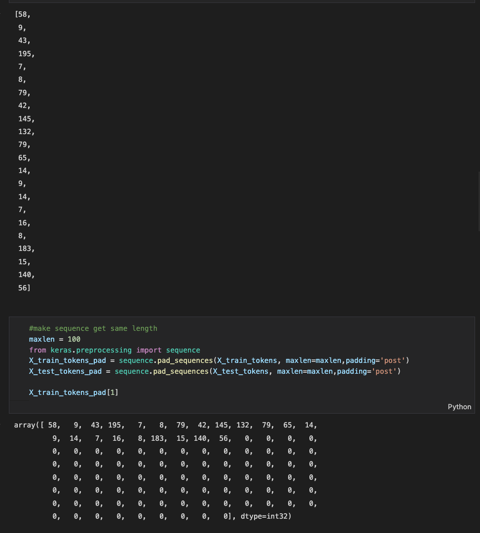
3. 搭建模型RNN/GRU/LSTM
#build model
embeddings_dim = 30
from keras.models import Model, Sequential
from keras.layers import Embedding, LSTM, GRU, SimpleRNN, Dense
#pick model, 0:RNN, 1:GRU, 2:LSTM
model_list = ['RNN','GRU','LSTM']

def buildModel(int:max_words,embeddings_dim,maxlen, model_pick):
  model = Sequential()
  model.add(Embedding(input_dim = max_words,
                      output_dim = embeddings_dim,
                      input_length=maxlen))
  #change model
  if model_pick == 'RNN':
    model.add(SimpleRNN(units=64))
  elif model_pick == 'GRU':
    model.add(GRU(units=64))
  elif model_pick == 'LSTM':
    model.add(LSTM(units=64))
  #activation function, we use sigmoid
  model.add(Dense(units=1, activation='sigmoid'))

  return model

#check both model
#RNN
model_pick = model_list[0]
RNNmodel = buildModel(max_words,embeddings_dim,maxlen,model_pick)
RNNmodel.summary()
#GRU
model_pick = model_list[1]
GRUmodel = buildModel(max_words,embeddings_dim,maxlen,model_pick)
GRUmodel.summary()
#LSTM
model_pick = model_list[2]
LSTMmodel = buildModel(max_words,embeddings_dim,maxlen,model_pick)
LSTMmodel.summary()

Model: "sequential_3"
_________________________________________________________________
 Layer (type)                Output Shape              Param #
=================================================================
 embedding_3 (Embedding)     (None, 100, 30)           6000

 simple_rnn_1 (SimpleRNN)    (None, 64)                6080

 dense_3 (Dense)             (None, 1)                 65

=================================================================
Total params: 12,145
Trainable params: 12,145
Non-trainable params: 0
_________________________________________________________________
Model: "sequential_4"
_________________________________________________________________
 Layer (type)                Output Shape              Param #
=================================================================
 embedding_4 (Embedding)     (None, 100, 30)           6000

 gru_1 (GRU)                 (None, 64)                18432

 dense_4 (Dense)             (None, 1)                 65

=================================================================
Total params: 24,497
Trainable params: 24,497
Non-trainable params: 0
_________________________________________________________________
Model: "sequential_5"
_________________________________________________________________
 Layer (type)                Output Shape              Param #
=================================================================
 embedding_5 (Embedding)     (None, 100, 30)           6000

 lstm_1 (LSTM)               (None, 64)                24320

 dense_5 (Dense)             (None, 1)                 65

=================================================================
Total params: 30,385
Trainable params: 30,385
Non-trainable params: 0
_________________________________________________________________
模型介绍
1. RNN
为什么需要RNN(循环神经网络)
他们都只能单独的取处理一个个的输入,前一个输入和后一个输入是完全没有关系的。但是,某些任务需要能够更好的处理序列的信息,即前面的输入和后面的输入是有关系的。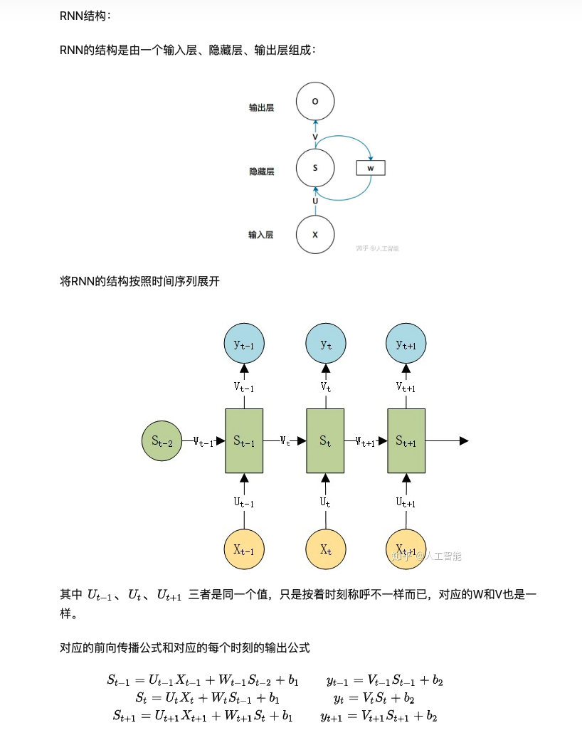
x是一个向量,它表示输入层的值(这里面没有画出来表示神经元节点的圆圈);s是一个向量,它表示隐藏层的值(这里隐藏层面画了一个节点,你也可以想象这一层其实是多个节点,节点数与向量s的维度相同);
U是输入层到隐藏层的权重矩阵,o也是一个向量,它表示输出层的值;V是隐藏层到输出层的权重矩阵。
那么,现在我们来看看W是什么。循环神经网络的隐藏层的值s不仅仅取决于当前这次的输入x,还取决于上一次隐藏层的值s。权重矩阵 W就是隐藏层上一次的值作为这一次的输入的权重。

one-to-n 的结构可以处理的问题有:
- 从图像生成文字(image caption),此时输入的X就是图像的特征,而输出的y序列就是一段句子,就像看图说话等
- 从类别生成语音或音乐等
n-to-one的结构:
这种结构通常用来处理序列分类问题。如输入一段文字判别它所属的类别,输入一个句子判断其情感倾向,输入一段视频并判断它的类别等等。
n-to-n结构:
最经典的RNN结构,输入、输出都是等长的序列数据。
n-to-m(Encoder-Decoder):
还有一种是 n-to-m,输入、输出为不等长的序列。
这种结构是Encoder-Decoder,也叫Seq2Seq,是RNN的一个重要变种。原始的n-to-n的RNN要求序列等长,然而我们遇到的大部分问题序列都是不等长的,如机器翻译中,源语言和目标语言的句子往往并没有相同的长度。为此,Encoder-Decoder结构先将输入数据编码成一个上下文语义向量c:
由于这种Encoder-Decoder结构不限制输入和输出的序列长度,因此应用的范围非常广泛,比如:
机器翻译:Encoder-Decoder的最经典应用,事实上这结构就是在机器翻译领域最先提出的。
文本摘要:输入是一段文本序列,输出是这段文本序列的摘要序列。
阅读理解:将输入的文章和问题分别编码,再对其进行解码得到问题的答案。
语音识别:输入是语音信号序列,输出是文字序列。
Encoder-Decoder 框架
Encoder-Decoder 不是一个具体的模型,是一种框架。
Encoder:将 input序列 →转成→ 固定长度的向量
Decoder:将 固定长度的向量 →转成→ output序列
Encoder 与 Decoder 可以彼此独立使用,实际上经常一起使用
因为最早出现的机器翻译领域,最早广泛使用的转码模型是RNN。其实模型可以是 CNN /RNN /BiRNN /LSTM /GRU /…
Encoder-Decoder 缺点
最大的局限性:编码和解码之间的唯一联系是固定长度的语义向量c
编码要把整个序列的信息压缩进一个固定长度的语义向量c
语义向量c无法完全表达整个序列的信息
先输入的内容携带的信息,会被后输入的信息稀释掉,或者被覆盖掉
输入序列越长,这样的现象越严重,这样使得在Decoder解码时一开始就没有获得足够的输入序列信息,解码效果会打折扣
因此,为了弥补基础的 Encoder-Decoder 的局限性,提出了attention机制。
2. LSTM
遗忘门
遗忘门的功能是决定应丢弃或保留哪些信息,来自前一个隐藏状态的信息和当前输入的信息同时传递到 sigmoid 函数中去,输出值介于 0 和 1 之间,越接近 0 意味着越应该丢弃,越接近 1 意味着越应该保留。
输入门
输入门的主要作用是更新细胞状态,首先将前一层隐藏状态的信息和当前输入的信息传递到sigmoid 函数中去,将值调整到 0~1 之间来决定要更新哪些信息。0 表示不更新,1 表示更新。其次还要将前一层隐藏状态的信息和当前输入的信息传递到 tanh 函数中去,创造一个新的候选值向量。最后将 sigmoid 的输出值与 tanh 的输出值相乘,sigmoid 的输出值将决定 tanh 的输出值中哪些信息是重要并且需要保留下来的。下图是输入门的具体运算过程。
输出门
输出门用来确定下一个隐藏状态的值,隐藏状态包含了先前输入的信息。首先,我们将前一个隐藏状态和当前输入传递到 sigmoid 函数中,然后将新得到的细胞状态传递给 tanh 函数。最后将 tanh 的输出与 sigmoid 的输出相乘,以确定隐藏状态应携带的信息。再将隐藏状态作为当前门的输出,把新的细胞状态和新的隐藏状态传递到下一个时间步长中去。
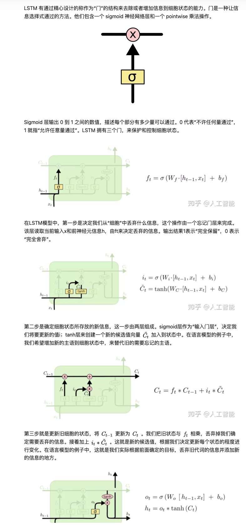
最后一步就是确定输出了,这个输出将会基于我们的细胞状态,但是也是一个过滤后的版本。首先,我们运行一个 sigmoid 层来确定细胞状态的哪个部分将输出出去。接着,我们把细胞状态通过 tanh 进行处理(得到一个在 -1 到 1 之间的值)并将它和 sigmoid 门的输出相乘,最终我们仅仅会输出我们确定输出的那部分。在语言模型的例子中,因为语境中有一个代词,可能需要输出与之相关的信息。例如,输出判断是一个动词,那么我们需要根据代词是单数还是负数,进行动词的词形变化。
3. GRU
与 LSTM 相比,GRU 去除掉了前面介绍的细胞状态部分,使用隐藏状态来进行信息的传递。因此它只包含两个门:更新门和重置门。
更新门
更新门的作用类似于 LSTM 中的遗忘门和输入门。它决定了要忘记哪些信息以及哪些新信息需要被添加
重置门
重置门用于决定遗忘先前信息的程度。另外,由于GRU的张量运算较少,因此它比 LSTM 的训练速度更快一些。但很难说这两者到底谁更好,只能说LSTM到目前为止比GRU更常用一些,具体可以根据实际的任务场景来选择。

4. 对比
RNN虽然擅长处理序列问题,但它也只能记住重要的短时信息,对于长时间的信息它则很难处理。也就是说,如果一条序列足够长,那它将很难把信息从较早的时间步传送到后面的时间步。因此,如果你准备进行一个文本预测任务,RNN 可能会遗漏一些间隔时间较长的重要信息。为什么会如此?因为RNN在反向传播的过程中,会面临梯度消失的问题,即梯度会随着时间推移慢慢下降。当梯度变得足够小,它就不会再进行学习。而LSTM和GRU就是短时记忆问题的解决方案。因为它们内部具有一些“门”可以调节信息流。这些“门”知道序列中哪些重要的数据是需要被保留,而哪些是需要被删除的。随后它可以沿着长链序列传递相关信息以进行预测,这也是为什么LSTM和GRU在后来的实际应用中越来越受欢迎的原因。
概括的来说,LSTM和GRU都能通过各种Gate将重要特征保留,保证其在long-term 传播的时候也不会被丢失。
标准LSTM和GRU的差别并不大,但是都比tanh要明显好很多,所以在选择标准LSTM或者GRU的时候还要看具体的任务是什么。
使用LSTM的原因之一是解决RNN Deep Network的Gradient错误累积太多,以至于Gradient归零或者成为无穷大,所以无法继续进行优化的问题。GRU的构造更简单:比LSTM少一个gate,这样就少几个矩阵乘法。在训练数据很大的情况下GRU能节省很多时间。
LSTM 的控制流程与 RNN 相似,都是在前向传播过程中处理流过节点的信息,不同之处在于 LSTM内部具有“门”结构,而各个“门”之间分工配合,更好地处理长时间的序列信息。其具体内部结构如下图所示。
4. 训练
#RNN
RNNmodel.compile(optimizer='adam',
                loss='binary_crossentropy',
                metrics=['accuracy'])
RNNhist = RNNmodel.fit(X_train, Y_train,
          callbacks=[metrics],
          validation_data=(X_test, Y_test),
          epochs=10,
          batch_size=128
          )
#plot training graph
from matplotlib import pyplot as plt
pd.DataFrame(RNNhist.history).plot(figsize=(10, 8))
plt.grid(True)
plt.show()

#GRU
GRUmodel.compile(optimizer='adam',
                loss='binary_crossentropy',
                metrics=['accuracy'])
GRUhist = GRUmodel.fit(X_train, Y_train,
          callbacks=[metrics],
          validation_data=(X_test, Y_test),
          epochs=10,
          batch_size=128
          )
#plot training graph
from matplotlib import pyplot as plt
pd.DataFrame(GRUhist.history).plot(figsize=(10, 8))
plt.grid(True)
plt.show()

#LSTM
LSTMmodel.compile(optimizer='adam',
                loss='binary_crossentropy',
                metrics=['accuracy'])
LSTMhist = LSTMmodel.fit(X_train, Y_train,
          callbacks=[metrics],
          validation_data=(X_test, Y_test),
          epochs=10,
          batch_size=128
          )
#plot training graph
from matplotlib import pyplot as plt
pd.DataFrame(LSTMhist.history).plot(figsize=(10, 8))
plt.grid(True)
plt.show()
LSTM取得最好结果
Adam优化器
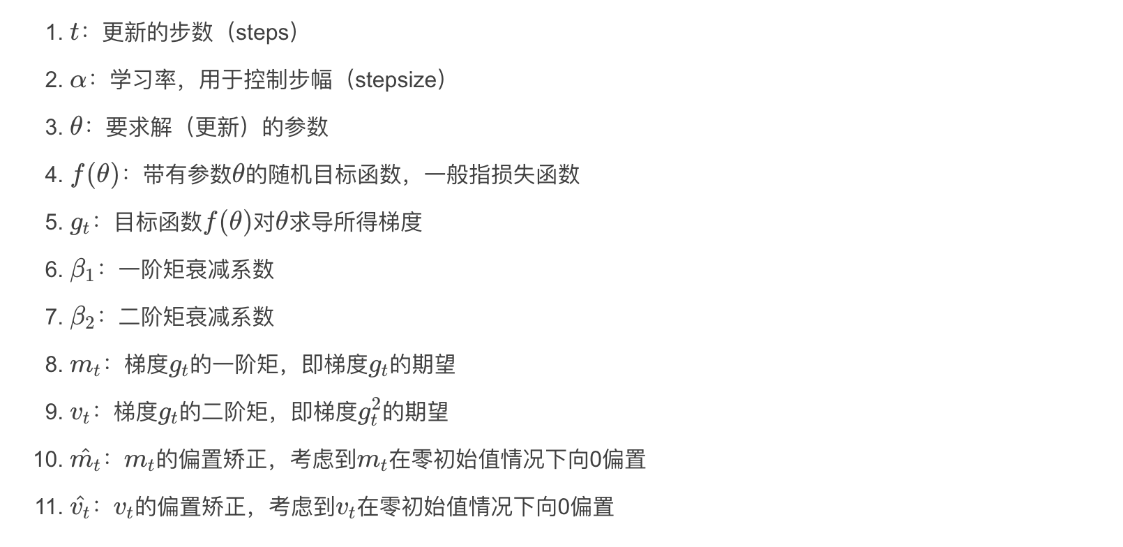
2014年12月,Kingma和Lei Ba两位学者提出了Adam优化器,结合AdaGrad和RMSProp两种优化算法的优点。对梯度的一阶矩估计(First Moment Estimation,即梯度的均值)和二阶矩估计(Second Moment Estimation,即梯度的未中心化的方差)进行综合考虑,计算出更新步长。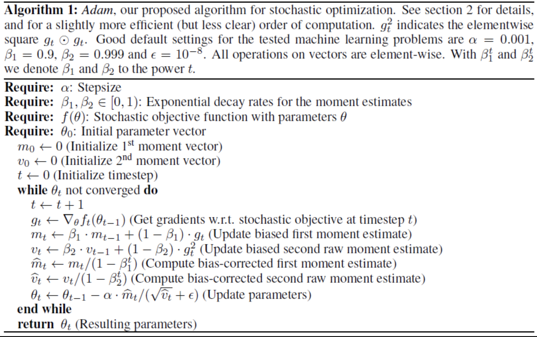

基于用户的英文评论的药品评级推荐系统
1. 数据集介绍
该数据集包含了一个药品推荐系统中用户对于各种药品的英文评论, 特征有药品名字,症状,评论,等级,点赞数
训练集包含了161 thousand条数据.
2. 数据处理
1. 数据清洗
首先查找数据中的脏数据,处理数据中的三种问题数据
1.在condition向量中存在爬虫错误数据,特点就是开头包涵
2.condition向量中存在nan数据
3.review评论向量中存在错误符号”'” 可根据ASCill表替换为”\’”
#######################################
# Explore data: preliminary analysis
#######################################

#we use excel to do the preliminary analysis
#we find out 'condition' columns includes bad data and blank data
#'reviewComment' also includes bad data

#check clounms
print(train.columns)

#check missing data
print(train.isna().sum())

#check duplicated values
#references: https://note.nkmk.me/en/python-pandas-duplicated-drop-duplicates/#:~:text=You%20can%20count%20the%20number,counted%20with%20sum()%20method.
print(train['uniqueID'].duplicated().sum())
#How many drug do we have?
print('repeated drugname is: '+ str(train['drugName'].duplicated().sum()))
print('length of drugname is: ' + str(len(train['drugName'].tolist())))
print('length of unique drugname is: ' + str(len(train['drugName'].unique().tolist())))

#Top popular drug
print(train['drugName'].value_counts().nlargest(5))

Index(['uniqueID', 'drugName', 'condition', 'review', 'rating', 'date',
       'usefulCount'],
      dtype='object')
uniqueID         0
drugName         0
condition      899
review           0
rating           0
date             0
usefulCount      0
dtype: int64
0
repeated drugname is: 157861
length of drugname is: 161297
length of unique drugname is: 3436
Levonorgestrel                       3657
Etonogestrel                         3336
Ethinyl estradiol / norethindrone    2850
Nexplanon                            2156
Ethinyl estradiol / norgestimate     2117
Name: drugName, dtype: int64
#fuchen 03/12/2022
#######################################
# Data cleaning
#######################################
##Cleaning1: replace the data in 'condition' column that contain '</span>' with blank
print('----------------cleaning 1 ---------------------------------')
count_train = 0
#Mode = the value that appears most frequently.
#references:https://pandas.pydata.org/docs/reference/api/pandas.DataFrame.mode.html
c = train['condition'].mode()[0]
vc = valid['condition'].mode()[0]
tc = test['condition'].mode()[0]
#for each error input of condition, esist </span>users found this comment helpful.,
#replace each error input to most frequently input
#count and clean train set:
for x in train.index:
if '</span>' in str(train.loc[x, 'condition']):
count_train +=1
train.loc[x, 'condition'] = c
#total 31 </span> in 'condition' col
print('Before clean, num of </span> in train is:' + str(count_train))
#check number of </span> again after cleaning
count_train = 0
for x in train.index:
if '</span>' in str(train.loc[ x, 'condition']) :
count_train +=1
print('After clean, num of </span> in train is:'+ str(count_train))
##############################################################
#count and clean valid set:
count_valid = 0
for x in valid.index:
if '</span>' in str(valid.loc[x, 'condition']):
count_valid +=1
valid.loc[x, 'condition'] = vc
#total 31 </span> in 'condition' col
print('Before clean, num of </span> in valid is:' + str(count_valid))
#check number of </span> again after cleaning
count_valid = 0
for x in valid.index:
if '</span>' in str(valid.loc[ x, 'condition']) :
count_valid +=1
print('After clean, num of </span> in valid is:'+ str(count_valid))
##############################################################
#count and clean test set:
count_test = 0
for x in test.index:
if '</span>' in str(test.loc[x, 'condition']):
count_test +=1
test.loc[x, 'condition'] = tc
#total 31 </span> in 'condition' col
print('Before clean, num of </span> in test is:' + str(count_test))
#check number of </span> again after cleaning
count_test = 0
for x in test.index:
if '</span>' in str(test.loc[ x, 'condition']) :
count_test +=1
print('After clean, num of </span> in test is:'+ str(count_test))
#Cleaning2: insert data into blank cell of 'condition' columns
print('----------------cleaning 2 ---------------------------------')
#references: https://datatofish.com/count-nan-pandas-dataframe/
#clean train set:
print('nan data in train[condition] is:'+ str(train['condition'].isna().sum()))
for i in train.index:
if pd.isna(train['condition'][i]) == True:
train.loc[i, 'condition'] = c
print('nan data in train[condition] after cleaning is:'+ str(train['condition'].isna().sum()))
#clean valid set:
print('nan data in valid[condition] is:'+ str(valid['condition'].isna().sum()))
for i in valid.index:
if pd.isna(valid['condition'][i]) == True:
valid.loc[i, 'condition'] = vc
print('nan data in valid[condition] after cleaning is:'+ str(valid['condition'].isna().sum()))
#clean test set:
print('nan data in test[condition] is:'+ str(test['condition'].isna().sum()))
for i in test.index:
if pd.isna(test['condition'][i]) == True:
test.loc[i, 'condition'] = tc
print('nan data in test[condition] after cleaning is:'+ str(test['condition'].isna().sum()))
#Cleaning3: replace the error code ''' in 'reviewComment' column with an apostrophe (’)
print('----------------cleaning 3 ---------------------------------')
def manually_cleanReview_train(data,count):
for i in data['review']:
if ''' in i :
count += 1
#total count''' need to be change to '\''
print('Before clean, num of ['] is:'+ str(count))
#replace ''' into (’)
data['review']=data.review.replace({"'": "\'"},regex=True)
#check number of ''' again after cleaning
count = 0
for i in data['review']:
if ''' in i :
count +=1
print('After clean, num of ['] is:'+ str(count))
def manually_cleanReview(data,count):
for i in data['reviewComment']:
if ''' in i :
count += 1
#total count''' need to be change to '\''
print('Before clean, num of ['] is:'+ str(count))
#replace ''' into (’)
data['reviewComment']=data.reviewComment.replace({"'": "\'"},regex=True)
#check number of ''' again after cleaning
count = 0
for i in data['reviewComment']:
if ''' in i :
count +=1
print('After clean, num of ['] is:'+ str(count))
count = 0
print('clean train[review]: ')
manually_cleanReview_train(train,count)
count = 0
print('clean valid[review]: ')
manually_cleanReview(valid,count)
#clean review in test:
count = 0
for i in test['reviewComment']:
if ''' in i :
count += 1
#total count''' need to be change to '\''
print('Before clean, num of ['] in test is:'+ str(count))
#replace ''' into (’)
test['reviewComment']=test.reviewComment.replace({"'": "\'"},regex=True)
#check number of ''' again after cleaning
count = 0
for i in test['reviewComment']:
if ''' in i :
count +=1
print('After clean, num of ['] in test is:'+ str(count))
----------------cleaning 1 ---------------------------------
Before clean, num of </span> in train is:900
After clean, num of </span> in train is:0
Before clean, num of </span> in valid is:8
After clean, num of </span> in valid is:0
Before clean, num of </span> in test is:13
After clean, num of </span> in test is:0
----------------cleaning 2 ---------------------------------
nan data in train[condition] is:899
nan data in train[condition] after cleaning is:0
nan data in valid[condition] is:5
nan data in valid[condition] after cleaning is:0
nan data in test[condition] is:9
nan data in test[condition] after cleaning is:0
----------------cleaning 3 ---------------------------------
clean train[review]:
Before clean, num of ['] is:100566
After clean, num of ['] is:0
clean valid[review]:
Before clean, num of ['] is:754
After clean, num of ['] is:0
Before clean, num of ['] in test is:1182
After clean, num of ['] in test is:0
2. 数据的特征提取
1. 数据不平衡
在condition变量中,数据分布不是正态分布会导致训练结果产生偏差
对数据分布稍微处理一下
#Since we notice condition are unbalanced,we need to balanced it
#fuchen 2021/3/23
#cleaning 4: removing low frequency class in condition
#check current class

print("Number of classes in train.condition: ", len(train["condition"].unique()))
print("Number of classes in valid.condition: ", len(valid["condition"].unique()))

# remove classes which have no more than 15 values in train
index_counts = train["condition"].value_counts()[train.condition.value_counts() >= 15].index
train = train[train["condition"].isin(index_counts)]
# remove classes which have no more than 15 values in validation
index_counts = valid["condition"].value_counts()[valid.condition.value_counts() >= 15].index
valid = valid[valid["condition"].isin(index_counts)]

print("Number of classes in train.condition after cleaned: ", len(train["condition"].unique()))
print("Number of classes in valid.condition after cleaned: ", len(valid["condition"].unique()))

# undersampling all classes with samples greater than 250 in train data set
condition_over250 = train["condition"].value_counts()[train.condition.value_counts() >= 250].index
# undersampling all classes with samples greater than 120 in valid data set
condition_over120 = valid["condition"].value_counts()[valid.condition.value_counts() >= 120].index
#for train
for x in condition_over250:
    # randomly shuffle the samples
    condition_samples = train[train["condition"]== x]
    condition_samples = condition_samples.sample(frac=1).reset_index(drop=True)

    # extract only 250
    condition_samples = condition_samples[:250]

    train = train[train["condition"] != x ]
    # put it back
    train = pd.concat([train, condition_samples], ignore_index=True)

#for validation:
for x in condition_over120:
    # randomly shuffle the samples
    condition_samples = valid[valid["condition"]== x]
    condition_samples = condition_samples.sample(frac=1).reset_index(drop=True)

    # extract only 220
    condition_samples = condition_samples[:120]

    valid = valid[valid["condition"] != x ]
    # put it back
    valid = pd.concat([valid, condition_samples], ignore_index=True)
处理后(这里应该有更好的处理方式,我这直接删除了频率最高的几类也不太正确):
2. TextBlob
微软开发的TextBlob库中的polarity函数可根据一段英文语意判断positive和negative并给出一个[0,1]的数,可以用来将review和condition转化为数字类型数据
#######################################
# Feature Extraction & Feature scaling
#######################################
#fuchen 2022/3/15
#Feature Extraction: the process of transforming raw data into numerical features that can be processed
# while preserving the information in the original data set.

#Feature scaling: Normalization typically means rescaling the values into similar range. e.g.[0,1]

#references:https://docs.microsoft.com/en-us/nimbusml/tutorials/b_a-sentiment-analysis-1-data-loading-with-pandas
#referneces: https://stackabuse.com/sentiment-analysis-in-python-with-textblob/
from textblob import TextBlob

def get_sentiment(txt):
  blob = TextBlob(txt)
  return blob.polarity

def get_sentiment_label(txt):
  blob = TextBlob(txt)
  if blob.polarity < -0.6:
    label = 'strongly negative, 1'
  elif blob.polarity >= -0.6 and blob.polarity < -0.2:
    label = 'negative, 2'
  elif blob.polarity >= -0.2 and blob.polarity < 0.2:
    label = 'neutral, 3'
  elif blob.polarity >= 0.2 and blob.polarity <0.6:
    label = 'positive, 4'
  elif blob.polarity >= 0.6:
    label = 'strongly positive, 5'
  return label
#According to documentation, the rating is mainly related to reviewComment
#Therefore, i turn reviewComment into numerical by sentiment Analysis
train['sentiment'] = train['review'].apply(get_sentiment)
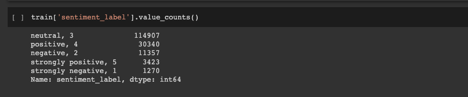
train['sentiment_label'] = train['review'].apply(get_sentiment_label)

#also turn valid data for later model training
valid['sentiment'] = valid['reviewComment'].apply(get_sentiment)
valid['sentiment_label'] = valid['reviewComment'].apply(get_sentiment_label)

#also turn test data
test['sentiment'] = test['reviewComment'].apply(get_sentiment)

#New, column 'reviewComment' turn into numerical
train.head()

#Feature scaling:
# we can do feature scaling to both usefulCount and rating
# x' = (x - min(x))/(max(x)-min(x))
train['usefulCount_scaling'] = (train.usefulCount - train.usefulCount.min()) / (train.usefulCount.max() - train.usefulCount.min())
train['rating_scaling'] = (train.rating - train.rating.min())/(train.rating.max() - train.rating.min())

train.head()

3. nltk(stopwords和SnowballStemmer)
nltk库中有两个函数可以帮助清洗复杂的长串英文字符.
首先import string,使用string.punctuation判别并去除标点符号,留下单词
在用stopwords去除介词、连词、代词
最后使用stemmer.stem(word)把每个单词恢复到现在时态并以小些输出
#######################################
# reviewComment tokenlization
#######################################
#fuchen 2022/3/23
#we use nltk to tokenlize some complex columns such as reviewComment and condition
#references: https://pythonspot.com/nltk-stop-words/
#reference: https://www.geeksforgeeks.org/snowball-stemmer-nlp/
#Download stopwords for clean reviewComment
nltk.download(['punkt','stopwords'])
import nltk
from nltk.corpus import stopwords
from nltk.stem import SnowballStemmer
import string
#Download stopwords for clean reviewComment
nltk.download(['punkt','stopwords'])

def FeatureExtraction(reviews):
  stop = stopwords.words('english')
  stemmer = SnowballStemmer("english")

  # remove punctuations, only english words
  reviews = reviews.str.replace('[{}]'.format(string.punctuation), '')
  # Remove stop words, such as a, an, the, high frequency prepositions, conjunctions, pronouns, etc.
  words = reviews.apply(
      lambda x: ' '.join([word for word in x.split() if word not in stop]))
  # turn word into original, e.g. word ‘stemmed‘ it is replaced with the word ‘stem‘
  stemming_words = words.apply(lambda x: ' '.join([stemmer.stem(word) for word in x.split()]))

  return stemming_words

#feature extraction review
train['clean_review'] = FeatureExtraction(train["review"]).str.lower()
valid["clean_review"] = FeatureExtraction(valid["reviewComment"]).str.lower()
test['clean_review'] = FeatureExtraction(test["reviewComment"]).str.lower()
4. one-hot
由于症状和药品名字两个变量有很多的相同情况,可以binary 分类为常见病和不常见
使用one-hot将其分类
#onehot in train drugname label
train_top_drug = list(train['drugName'].value_counts()[:500].index)
i = 0
for drug_name in train_top_drug:
    train['drugName_' + str(i)] = train['drugName'].apply(lambda x: 1 if drug_name in x else 0)
    i += 1
#train condition
train_top_condition = list(train['condition'].value_counts()[:150].index)
i = 0
for con in train_top_condition:
    train['condition_' + str(i)] = train['condition'].apply(lambda x: 1 if con in x else 0)
    i += 1

#valid drugName
valid_top_drug = list(valid['drugName'].value_counts()[:76].index)
i = 0
for drug_name in valid_top_drug:
    valid['drugName_' + str(i)] = valid['drugName'].apply(lambda x: 1 if drug_name in x else 0)
    i += 1
#valid condition
valid_top_condition = list(valid['condition'].value_counts()[:28].index)
i = 0
for con in valid_top_condition:
    valid['condition_' + str(i)] = valid['condition'].apply(lambda x: 1 if con in x else 0)
    i += 1

#test drugName
test_top_drug = list(test['drugName'].value_counts()[:94].index)
i = 0
for drug_name in test_top_drug:
    test['drugName_' + str(i)] = test['drugName'].apply(lambda x: 1 if drug_name in x else 0)
    i += 1
#test condition
test_top_condition = list(test['condition'].value_counts()[:36].index)
i = 0
for con in test_top_condition:
    test['condition_' + str(i)] = test['condition'].apply(lambda x: 1 if con in x else 0)
    i += 1
5. sklearn.TfIdf
使用python ml 开源库sklearn中的TfIdf函数算出词频,讲刚才处理好的评论变量中的所有英文单词变成数字方便训练
from sklearn.feature_extraction.text import TfidfVectorizer,CountVectorizer

# Creates TF-IDF vectorizer and transforms the corpus
vectorizer = TfidfVectorizer()
X_train = vectorizer.fit_transform(train.clean_review)
# transforms test reviews to above vectorized format
X_test = vectorizer.transform(valid.clean_review)
3. 模型搭建
- 贝叶斯分类器

from sklearn.naive_bayes import MultinomialNB
from sklearn.metrics import confusion_matrix
from sklearn.metrics import f1_score
#reference: https://hands-on.cloud/implementing-naive-bayes-classification-using-python/
#reference: https://scikit-learn.org/stable/modules/generated/sklearn.feature_extraction.text.TfidfVectorizer.html

#二分类或者按照rating分成5类
select_ratingLevel(2,X_train, X_test)
select_ratingLevel(5,X_train, X_test)

# Train Naïve Bayes classifier and make prediction
def bayesPred(X_train,X_test,y_train_rating):
  start = time.time()
  model1 = MultinomialNB()
  model1.fit(X_train, y_train_rating)
  end = time.time()
  print("Training time: %s" % str(end-start))
  pred_bayes = model1.predict(X_test)
  return model1, pred_bayes

def select_ratingLevel(choice,X_train,X_test):
  if choice == 2:
    # Create a column with binary rating with 1&2 as a class and 3&4&5 as a class indicating the polarity of a review
    train['binary_rating'] = train['rating'] > 2
    y_train_rating = train.binary_rating
    # Evaluates model on valid set with binary rating in valid set
    valid['binary_rating'] = valid.rating > 2
    y_valid_rating = valid.binary_rating
    #build bayes model and predict model
    model1, pred_bayes = bayesPred(X_train,X_test, y_train_rating)
    #output result
    print("validation Accuracy of binary rating is: %s" % str(model1.score(X_test, y_valid_rating)))
    macro_f1 = f1_score(pred_bayes, y_valid_rating, average='macro')
    micro_f1 = f1_score(pred_bayes, y_valid_rating, average='micro')
    print("validation Accuracy of binary rating in macro_f1 is: %s" % str(macro_f1))
    print("validation Accuracy of binary rating in micro_f1 is: %s" % str(micro_f1))
    print("Confusion Matrix")
    print(confusion_matrix(pred_bayes, y_valid_rating))
  if choice == 5:
    # Create a column with binary rating with 5 classes indicating the polarity of a review
    y_train_rating = train.rating
    # Evaluates model on valid set with 5 class rating in valid set
    y_valid_rating = valid.rating
    #build bayes model and predict model
    model1, pred_bayes = bayesPred(X_train,X_test, y_train_rating)
    #output result
    print("validation Accuracy of 5-class rating is: %s" % str(model1.score(X_test, y_valid_rating)))
    macro_f1 = f1_score(pred_bayes, y_valid_rating, average='macro')
    micro_f1 = f1_score(pred_bayes, y_valid_rating, average='micro')
    print("validation Accuracy of 5-class rating in macro_f1 is: %s" % str(macro_f1))
    print("validation Accuracy of 5-class rating in micro_f1 is: %s" % str(micro_f1))
    print("Confusion Matrix")
    print(confusion_matrix(pred_bayes, y_valid_rating))
- 随机森林randomforest
from sklearn.ensemble import RandomForestClassifier
#fuchen 2022/3/25
#reference: https://scikit-learn.org/stable/modules/generated/sklearn.ensemble.RandomForestClassifier.html

def randomForest(X_train, y_train_rating):
  # Trains random forest classifier
  start = time.time()
  rfc_rating = RandomForestClassifier(
                                      n_estimators=100,        # number of tree--100 tree build
                                      random_state=50,          # random level
                                      max_depth = None,         # max depth of each tree
                                      min_samples_split = 0.001, # minimum number of samples required to split an internal node
                                      )

  rfc_rating.fit(X_train, y_train_rating)
  end = time.time()
  print("Training time: %s" % str(end-start))
  return rfc_rating

def select_classRating(choice,X_train,X_test):
  if choice == 2:
    # Create a column with binary rating with 1&2 as a class and 3&4&5 as a class indicating the polarity of a review
    train['binary_rating'] = train['rating'] > 2
    y_train_rating = train.binary_rating
    # Evaluates model on valid set with binary rating in valid set
    valid['binary_rating'] = valid.rating > 2
    y_valid_rating = valid.binary_rating

    #build model
    rfc_rating = randomForest(X_train, y_train_rating)

    #output result
    # Evaluates model on test set
    pred_random_forest = rfc_rating.predict(X_test)
    print("validation Accuracy of binary rating is: %s" % str(rfc_rating.score(X_test, y_valid_rating)))
    macro_f1 = f1_score(pred_random_forest, y_valid_rating, average='macro')
    micro_f1 = f1_score(pred_random_forest, y_valid_rating, average='micro')
    print("validation Accuracy of binary rating in macro_f1 is: %s" % str(macro_f1))
    print("validation Accuracy of binary rating in micro_f1 is: %s" % str(micro_f1))
    print("Confusion Matrix")
    print(confusion_matrix(pred_random_forest, y_valid_rating))
  if choice == 5:
    # Create a column with binary rating with 5 classes indicating the polarity of a review
    y_train_rating = train.rating
    # Evaluates model on valid set with 5 class rating in valid set
    y_valid_rating = valid.rating
    #build model
    rfc_rating = randomForest(X_train, y_train_rating)
    #output result
    # Evaluates model on validation set
    pred_random_forest = rfc_rating.predict(X_test)
    print("validation Accuracy of 5 class rating is: %s" % str(rfc_rating.score(X_test, y_valid_rating)))
    macro_f1 = f1_score(pred_random_forest, y_valid_rating, average='macro')
    micro_f1 = f1_score(pred_random_forest, y_valid_rating, average='micro')
    print("validation Accuracy of 5 class rating in macro_f1 is: %s" % str(macro_f1))
    print("validation Accuracy of 5 class rating in micro_f1 is: %s" % str(micro_f1))
    print("Confusion Matrix")
    print(confusion_matrix(pred_random_forest, y_valid_rating))


def main():
  # references: https://scikit-learn.org/stable/modules/generated/sklearn.feature_extraction.text.TfidfVectorizer.html
  # Creates TF-IDF vectorizer and transforms the corpus
  vectorizer = TfidfVectorizer()
  X_train = vectorizer.fit_transform(train.clean_review)
  # transforms test reviews to above vectorized format
  X_test = vectorizer.transform(valid.clean_review)
  #select binary rating input 2 and 5 rating input 5
  select_classRating(2,X_train, X_test)
  select_classRating(5,X_train, X_test)

main()
- XgBoost
从xgboost库中导入XGBClassifier分类器
#fuchen 2022/3/15
from sklearn.metrics import f1_score
from sklearn.metrics import accuracy_score
from xgboost import XGBClassifier
from xgboost import plot_importance
#reference:https://www.datatechnotes.com/2019/07/classification-example-with.html
def xgBoost(X_train, y_train_rating):
  # Trains random forest classifier
  start = time.time()
  xgb_model = XGBClassifier(learning_rate=0.001,         # Controls the step size when updating the weights each iteration
                             n_estimators=200,         # number of tree--100 tree build xgboost
                             max_depth=6,               # depth of tree
                             min_child_weight = 1,      # min weight of child node
                             gamma=0.,                  # The parameter before the number of child nodes in the penalty term
                             subsample=0.8,             # Randomly select 80% of the samples to build a decision tree
                             colsample_btree=0.8,       # Randomly select 80% of the features to build a decision tree
                             objective='multi:softmax', # define loss function
                             scale_pos_weight=1,        # solve unbalanced sample size
                             random_state=27            # random level
                             )
  xgb_model.fit(X_train, y_train_rating)
  end = time.time()
  print("Training time: %s" % str(end-start))
  return xgb_model

def select_classRating(X_train,X_test):
  # Create a column with binary rating with 5 classes indicating the polarity of a review
  y_train_rating = train.rating
  # Evaluates model on valid set with 5 class rating in valid set
  y_valid_rating = valid.rating

  #build model
  xgb_model = xgBoost(X_train, y_train_rating)

  #output result
  # Evaluates model on test set
  pred_xgBoost = xgb_model.predict(X_test)

  print("Accuracy of 5 class rating is: %s" % str(xgb_model.score(X_test, y_valid_rating)))
  macro_f1 = f1_score(pred_xgBoost, y_valid_rating, average='macro')
  micro_f1 = f1_score(pred_xgBoost, y_valid_rating, average='micro')
  print("Accuracy of 5 class rating in macro_f1 is: %s" % str(macro_f1))
  print("Accuracy of 5 class rating in micro_f1 is: %s" % str(micro_f1))
  print("Confusion Matrix")
  print(confusion_matrix(pred_xgBoost, y_valid_rating))

  return pred_xgBoost

def main():
  # references: https://scikit-learn.org/stable/modules/generated/sklearn.feature_extraction.text.TfidfVectorizer.html
  # Creates TF-IDF vectorizer and transforms the corpus
  vectorizer = TfidfVectorizer()
  X_train = vectorizer.fit_transform(train.clean_review)
  # transforms test reviews to above vectorized format
  X_test = vectorizer.transform(valid.clean_review)
  #build model and training
  xgb_preds_test = select_classRating(X_train, X_test)

main()
- CNN
#use keras's Tokenizer function to transfer sentences into tokens
from keras.preprocessing.text import Tokenizer
import numpy
from keras.preprocessing.sequence import pad_sequences
from torch.nn.utils.rnn import pad_sequence
import torch
from torch import nn
import torch.nn.functional as F
from sklearn.metrics import f1_score
from sklearn.metrics import accuracy_score


#split data
X_train = train_df['clean_review']
X_valid = valid['clean_review']
y_train = train_df['rating']
y_valid = valid['rating']
X_test = test['clean_review']


embed_size = 300
max_features = 120000
maxlen = 750 # max number of words in a question to use
batch_size = 500 # how many samples to process at once

# n_splits = 5 # Number of K-fold Splits
# SEED = 10
debug = 0
## Tokenize the sentences
tokenizer = Tokenizer(num_words=max_features)
tokenizer.fit_on_texts(X_train)

X_train = tokenizer.texts_to_sequences(X_train)
X_valid = tokenizer.texts_to_sequences(X_valid)
X_test = tokenizer.texts_to_sequences(X_test)

## Pad the sentences
X_train = pad_sequences(X_train, maxlen=maxlen)
X_valid = pad_sequences(X_valid, maxlen=maxlen)
X_test = pad_sequences(X_test, maxlen=maxlen)

from sklearn.preprocessing import LabelEncoder
le = LabelEncoder()
y_train = le.fit_transform(y_train.values)
y_valid = le.transform(y_valid.values)
le.classes_

#word embedding
def load_glove(word_index):
    EMBEDDING_FILE = '/content/drive/MyDrive/5434project/glove.840B.300d.txt'
    def get_coefs(word,*arr): return word, np.asarray(arr, dtype='float32')[:300]
    embeddings_index = dict(get_coefs(*o.split(" ")) for o in open(EMBEDDING_FILE))

    all_embs = np.stack(embeddings_index.values())
    emb_mean,emb_std = -0.005838499,0.48782197
    embed_size = all_embs.shape[1]

    nb_words = min(max_features, len(word_index)+1)
    embedding_matrix = np.random.normal(emb_mean, emb_std, (nb_words, embed_size))
    for word, i in word_index.items():
        if i >= max_features: continue
        embedding_vector = embeddings_index.get(word)
        if embedding_vector is not None:
            embedding_matrix[i] = embedding_vector
        else:
            embedding_vector = embeddings_index.get(word.capitalize())
            if embedding_vector is not None:
                embedding_matrix[i] = embedding_vector
    return embedding_matrix


if debug:
    embedding_matrix = np.random.randn(120000,300)
else:
    embedding_matrix = load_glove(tokenizer.word_index)


#2022/3/31
# The size of each convolution kernel is filter_size*embedding_size.
# filter_size represents the number of words that the convolution kernel contains vertically,
# that is, it is considered that there is a word order relationship between adjacent words,

# After each convolution kernel is calculated, we get a column vector,
# which represents the features extracted by the convolution kernel from the sentence.
# How many kinds of features can be extracted by how many convolution kernels,
# that is, the number of channels in the depth direction in the figure.
class CNN_Text(nn.Module):

    def __init__(self):
        super(CNN_Text, self).__init__()
        #[5,4,3,2,1] is used in the code. embedding_size is the dimension of the word vector.
        filter_sizes = [5,4,3,2,1]
        num_filters = 28
        # embedding layer, which maps vocabulary indices to low-dimensional word vectors for representation.
        # It is essentially a vector table of words that we learn from the data.
        self.embedding = nn.Embedding(max_features, embed_size)
        self.embedding.weight = nn.Parameter(torch.tensor(embedding_matrix, dtype=torch.float32))
        self.embedding.weight.requires_grad = False
        # Convolutional layers
        self.convs1 = nn.ModuleList([nn.Conv2d(1, num_filters, (i, embed_size)) for i in filter_sizes])
        #Reduce overfitting
        self.dropout = nn.Dropout(0.1)
        # fully connected layer
        self.fc1 = nn.Linear(len(filter_sizes)*num_filters, 5)


    def forward(self, x):
        x = self.embedding(x)
        x = x.unsqueeze(1)
        x = [F.relu(conv(x)).squeeze(3) for conv in self.convs1]
        x = [F.max_pool1d(i, i.size(2)).squeeze(2) for i in x]
        x = torch.cat(x, 1)
        x = self.dropout(x)
        logit = self.fc1(x)
        return logit

n_epochs = 6
model = CNN_Text()
loss_fn = nn.CrossEntropyLoss(reduction='sum')
optimizer = torch.optim.Adam(filter(lambda p: p.requires_grad, model.parameters()), lr=0.001)
model

# Load train and test
x_train = torch.tensor(X_train, dtype=torch.long)
y_train = torch.tensor(y_train, dtype=torch.long)

x_cv = torch.tensor(X_valid, dtype=torch.long)
y_cv = torch.tensor(y_valid, dtype=torch.long)

x_test = torch.tensor(X_test, dtype=torch.long)
# Create Torch datasets
train = torch.utils.data.TensorDataset(x_train, y_train)
valid = torch.utils.data.TensorDataset(x_cv, y_cv)

# Create Data Loaders
train_loader = torch.utils.data.DataLoader(train, batch_size=batch_size, shuffle=True)
valid_loader = torch.utils.data.DataLoader(valid, batch_size=batch_size, shuffle=False)
test_rating_list = []
train_loss = []
valid_loss = []
#training
epochs = 6

for epoch in range(epochs):
    epoch_loss = 0
    epoch_accuracy = 0

    for data, label in train_loader:
        output = model(data)
        loss = loss_fn(output, label)

        optimizer.zero_grad()
        loss.backward()
        optimizer.step()

        acc = ((output.argmax(dim=1) == label).float().mean())
        epoch_accuracy += acc/len(train_loader)
        epoch_loss += loss/len(train_loader)

    print('Epoch : {}, train accuracy : {}, train loss : {}'.format(epoch+1, epoch_accuracy,epoch_loss))

    with torch.no_grad():
        epoch_val_accuracy=0
        epoch_val_loss =0
        for data, label in valid_loader:
            val_output = model(data)
            val_loss = loss_fn(val_output,label)


            acc = ((val_output.argmax(dim=1) == label).float().mean())
            epoch_val_accuracy += acc/ len(valid_loader)
            epoch_val_loss += val_loss/ len(valid_loader)

        print('Epoch : {}, val_accuracy : {}, val_loss : {}'.format(epoch+1, epoch_val_accuracy,epoch_val_loss))

    with torch.no_grad():
        for data, label in test_loader:
            test_output = model(data)
            test_rating_list.append(test_output.argmax(dim=1))
4. 数据可视化
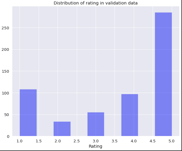
- EDA figures
相关矩阵correlation matrix显示出sentiment(review)这个变量和被预测的rating最相关


- word cloud ```python
from wordcloud import WordCloud, STOPWORDS
reference: https://www.kaggle.com/aashita/word-clouds-of-various-shapes
def plot_wordcloud(text, mask=None, max_words=200, max_font_size=100, figure_size=(24.0,16.0), title = None, title_size=40, image_color=False): stopwords = set(STOPWORDS) more_stopwords = {‘one’, ‘br’, ‘Po’, ‘th’, ‘sayi’, ‘fo’, ‘Unknown’} stopwords = stopwords.union(more_stopwords)
wordcloud = WordCloud(background_color='white',
                stopwords = stopwords,
                max_words = max_words,
                max_font_size = max_font_size,
                random_state = 42,
                width=800,
                height=400,
                mask = mask)
wordcloud.generate(str(text))

plt.figure(figsize=figure_size)
if image_color:
    image_colors = ImageColorGenerator(mask);
    plt.imshow(wordcloud.recolor(color_func=image_colors), interpolation="bilinear");
    plt.title(title, fontdict={'size': title_size,
                              'verticalalignment': 'bottom'})
else:
    plt.imshow(wordcloud);
    plt.title(title, fontdict={'size': title_size, 'color': 'black',
                              'verticalalignment': 'bottom'})
plt.axis('off');
plt.tight_layout()
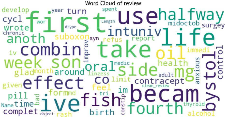
plot_wordcloud(train_df[“clean_review”], title=”Word Cloud of review”)
<a name="Ik28T"></a>
## 4. 训练
---
<a name="d3L1p"></a>
# 猫狗照片识别基于自己建立的简单5层CNN网络模型
<a name="WTiiE"></a>
## 1. 数据集介绍
训练集包含8003张猫和狗的jpg图片,验证集有2023张.结尾是有*.jpg组成.由于猫和狗的图片分开在不同的文件夹,因此我们使用glob从文件夹中读取所有猫和狗图merge在一起<br />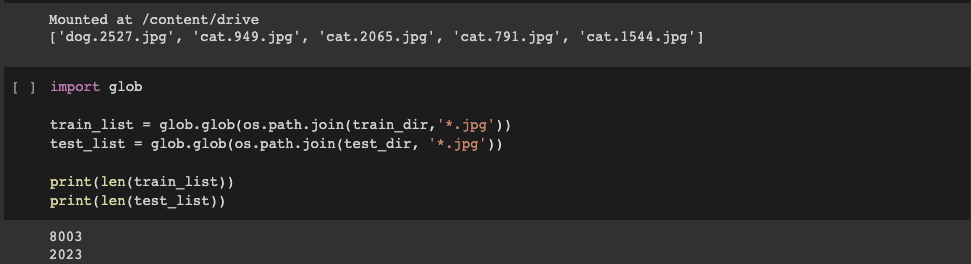<br />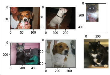
<a name="UdWW8"></a>
## 2. 数据处理
我写了两种版本,一种Pytorch一种tensorflow
<a name="ts7CI"></a>
### Pytorch:
由于每个图片的大小都不一样,我们需要裁剪图片为一样的维度大小.<br />首先使用sklearn库中的train——test——split函数将训练集按照8/2分成训练集和测试集.<br />由于使用pytorch,需要使用torchvision库中的transforms函数将图片转化
1. resize函数缩放图片
1. RandomResizedCrop函数根据中心切割图片
1. RandomHorizontalFilp函数水平旋转
1. ToTensor函数将图片变成pytorch可训练的特征矩阵
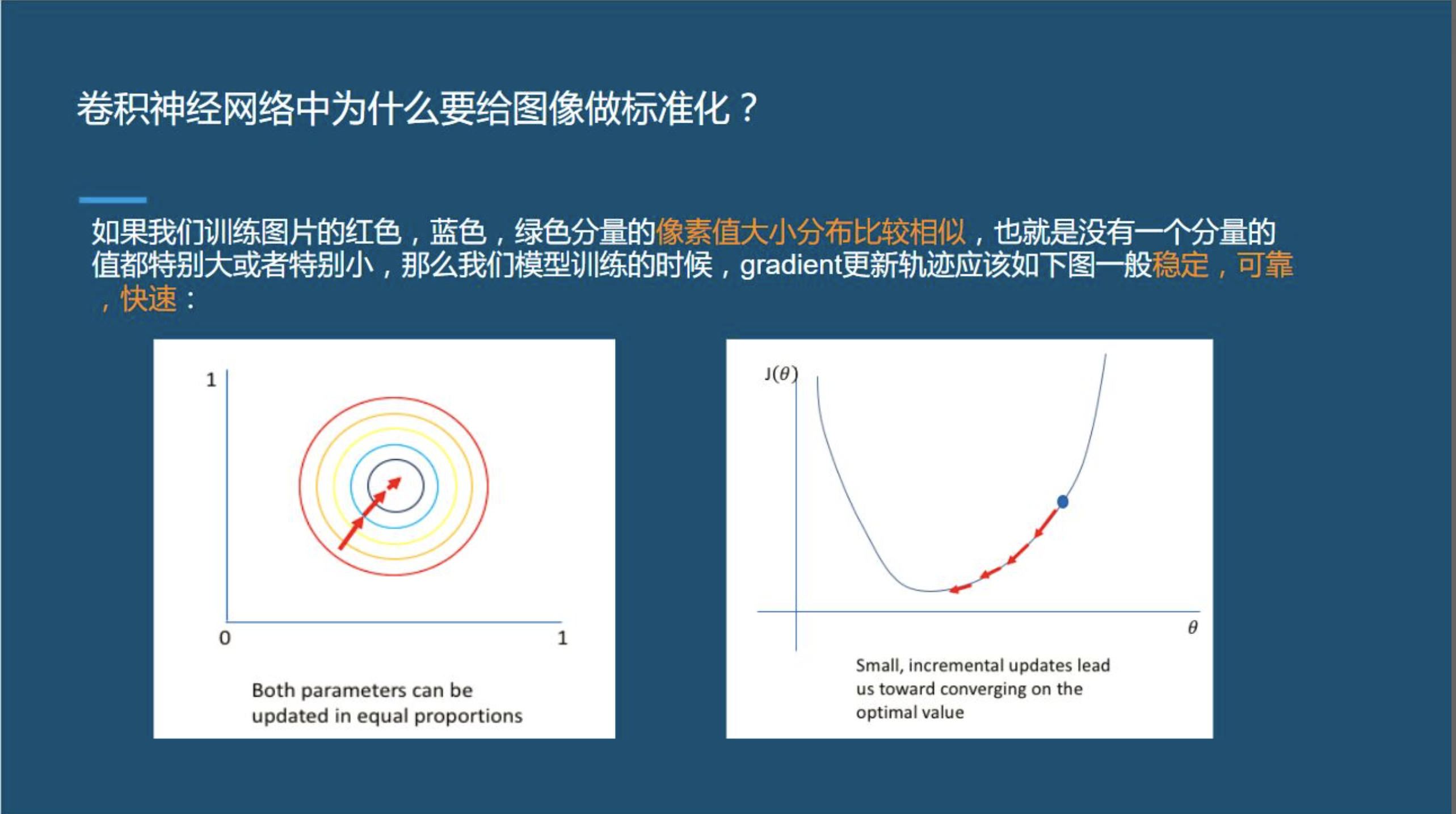
1. Normalize函数标准化,由于图片是RGB三个维度,如果三个颜色不平衡会导致后期训练梯度消失/爆炸问题
6. 接着把处理好的图片所形成特征矩阵装进torch库中的dataset里,再使用DataLoader将数据打包成batch_size=64的大小方便训练.
```python
#import all necessary Libraries
#about torch...
import torch
import torch.nn as nn
import torch
import torch.optim as optim
import torch.nn.functional as F
from torchvision import datasets, models, transforms
from torch.utils.data import DataLoader, Dataset
#using numpy
import numpy as np
#split train set into train and validation set with 80% and 20%
from sklearn.model_selection import train_test_split
train_list, val_list = train_test_split(train_list, test_size=0.2)
#data feature extraction and cleaning
#transform figures into same size tensor for training, b/c every figure are different size
train_transforms = transforms.Compose([
#resize figure
transforms.Resize((255, 255)),
# Cut the image randomly into 224 square pictures according to the center
transforms.RandomResizedCrop(224),
# Flip horizontally with probability
transforms.RandomHorizontalFlip(),
# turn into tensor for directly training in model
transforms.ToTensor(),
# normalize data
transforms.Normalize((0.5, 0.5, 0.5), (0.5, 0.5, 0.5))
])
val_transforms = transforms.Compose([
transforms.Resize((255, 255)),
transforms.RandomResizedCrop(224),
transforms.RandomHorizontalFlip(),
transforms.ToTensor(),
transforms.Normalize((0.5, 0.5, 0.5), (0.5, 0.5, 0.5))
])
test_transforms = transforms.Compose([
transforms.Resize((255, 255)),
transforms.RandomResizedCrop(224),
transforms.RandomHorizontalFlip(),
transforms.ToTensor(),
transforms.Normalize((0.5, 0.5, 0.5), (0.5, 0.5, 0.5))
])
train_data = dataset(train_list, transform=train_transforms)
test_data = dataset(test_list, transform=test_transforms)
val_data = dataset(val_list, transform=test_transforms)
train_loader = torch.utils.data.DataLoader(dataset = train_data, batch_size=64, shuffle=True )
test_loader = torch.utils.data.DataLoader(dataset = test_data, batch_size=64, shuffle=True)
val_loader = torch.utils.data.DataLoader(dataset = val_data, batch_size=64, shuffle=True)
#check our images shape
train_data[0][0].shape
Tensorflow:
使用tensorflow.keras库中的ImageDataGenerator将图片缩放成统一大小255x255x3
接着直接使用ImageDataGenerator.flow_from_directory函数将数据打包成batch=32的大小
flow_from_directory(directory): 以文件夹路径为参数,生成经过数据提升/归一化后的数据,在一个无限循环中无限产生batch数据,
- target_size: 整数tuple,默认为(256, 256). 图像将被resize成该尺寸
- calss_mode: “binary” 将是 1D 二进制标签,”sparse” 将是 1D 整数标签,”categorical” 将是 2D one-hot 编码标签,”input” 将是与输入图像相同的图像(主要用于自动编码器)。
```python
importing libraries
import pandas as pd import numpy as np import matplotlib.pyplot as plt import tensorflow as tf import os from tensorflow.keras.preprocessing import imageimporting libraries for Deep Learning
from tensorflow.keras.models import Sequential from tensorflow.keras.layers import Conv2D, MaxPooling2D, Flatten, Dense, Dropout, Activation from tensorflow.keras.preprocessing.image import ImageDataGenerator from tensorflow.keras.optimizers import Adam
connect to google drive
from google.colab import drive drive.mount(‘/content/drive’)
train_dir = ‘/content/drive/MyDrive/training_set’ test_dir = ‘/content/drive/MyDrive/test_set’
transfer images intp array of numbers
references: https://keras.io/api/preprocessing/image/
since our data are label into 2 folders cats and dogs, wo we choice use
data_generator.flow_from_directory that can directly read data in two floders
data_generator = ImageDataGenerator(rescale = 1.0/255.0, zoom_range = 0.2)
batch_size = 32 training_data = data_generator.flow_from_directory(directory = train_dir, target_size = (64, 64), batch_size = batch_size, class_mode = ‘binary’) testing_data = data_generator.flow_from_directory(directory = test_dir, target_size = (64, 64), batch_size = batch_size, class_mode = ‘binary’)
<a name="Gxlo9"></a>
## 3. 搭建模型
<a name="GQ3nr"></a>
### Pytorch:
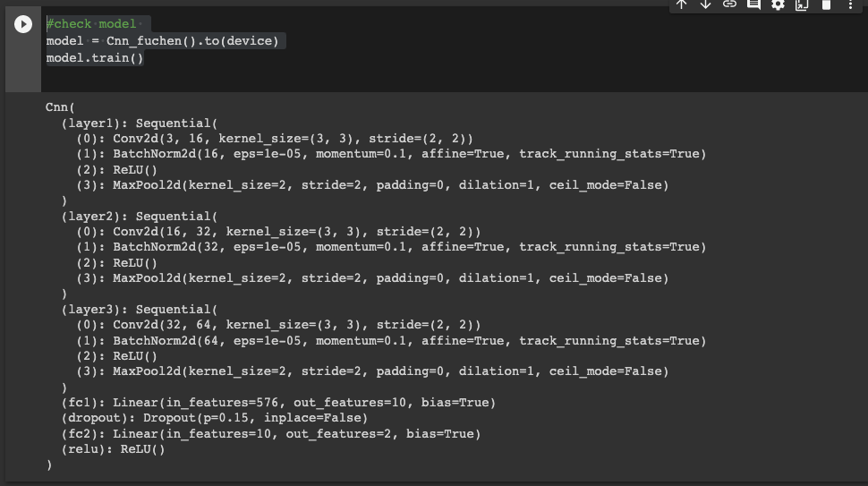
搭建一个简单5层网络,3层卷积层+2层全连阶层,加入batchNormalization和dropout防止过拟合可以多训练几个回合
```python
class Cnn_fuchen(nn.Module):
    def __init__(self):
        super(Cnn_fuchen,self).__init__()

        self.layer1 = nn.Sequential(
            nn.Conv2d(3,16,kernel_size=3, padding=0,stride=2),
            nn.BatchNorm2d(16),
            nn.ReLU(),
            nn.MaxPool2d(2)
        )

        self.layer2 = nn.Sequential(
            nn.Conv2d(16,32, kernel_size=3, padding=0, stride=2),
            nn.BatchNorm2d(32),
            nn.ReLU(),
            nn.MaxPool2d(2)
            )

        self.layer3 = nn.Sequential(
            nn.Conv2d(32,64, kernel_size=3, padding=0, stride=2),
            nn.BatchNorm2d(64),
            nn.ReLU(),
            nn.MaxPool2d(2)
        )

        self.fc1 = nn.Linear(3*3*64,10)
        self.dropout = nn.Dropout(0.15)
        self.fc2 = nn.Linear(10,2)
        self.relu = nn.ReLU()

    def forward(self,x):
        out = self.layer1(x)
        out = self.layer2(out)
        out = self.layer3(out)

        out = out.view(out.size(0),-1)
        out = self.relu(self.fc1(out))
        out = self.fc2(out)
        # x = torch.nn.functional.log_softmax(x,dim=1) # only NLLLoss()needed,crossentropy did not needed
        return out
Tensorflow:
卷积核为3x3, 3层卷积层+3层全连接层
def CNNmodel(data):

  #layer1
  model = Sequential()
  #activation function
  model.add(Conv2D(filters = 32, kernel_size = (3, 3), activation = 'relu', input_shape = data.image_shape))
  #maxpooling
  model.add(MaxPooling2D(pool_size = (2, 2)))


  #layer2
  model.add(Conv2D(filters = 64, kernel_size = (3, 3), activation = 'relu'))
  model.add(MaxPooling2D(pool_size = (2, 2)))

  #layer3
  model.add(Conv2D(filters = 128, kernel_size = (3, 3), activation = 'relu'))
  model.add(MaxPooling2D(pool_size = (2, 2)))


  model.add(Flatten())
  model.add(Dense(units = 128, activation = 'relu'))
  #dropout to avoid overfitting
  model.add(Dropout(rate = 0.2))
  model.add(Dense(units = 32, activation = 'relu'))
  # model.add(Dropout(rate = 0.1))

  model.add(Dense(units = 2, activation = 'sigmoid'))
  #optimizer, binary_crossentropy, sparse_categorical_crossentropy
  opt = Adam(lr=0.001)
  model.compile(optimizer = opt, loss = 'sparse_categorical_crossentropy', metrics = ['accuracy'])
  return model

model = CNNmodel(training_data)
model.summary()
Found 8005 images belonging to 2 classes.
Found 2023 images belonging to 2 classes.
Model: "sequential_8"
_________________________________________________________________
 Layer (type)                Output Shape              Param #
=================================================================
 conv2d_24 (Conv2D)          (None, 62, 62, 32)        896

 max_pooling2d_16 (MaxPoolin  (None, 31, 31, 32)       0
 g2D)

 conv2d_25 (Conv2D)          (None, 29, 29, 64)        18496

 max_pooling2d_17 (MaxPoolin  (None, 14, 14, 64)       0
 g2D)

 conv2d_26 (Conv2D)          (None, 12, 12, 128)       73856

 max_pooling2d_18 (MaxPoolin  (None, 6, 6, 128)        0
 g2D)

 flatten_8 (Flatten)         (None, 4608)              0

 dense_24 (Dense)            (None, 128)               589952

 dropout_17 (Dropout)        (None, 128)               0

 dense_25 (Dense)            (None, 32)                4128

 dense_26 (Dense)            (None, 2)                 66

=================================================================
Total params: 687,394
Trainable params: 687,394
Non-trainable params: 0
- Convolutional_1 : ((kernel_size)_stride+1)_filters) = (3_3_3+1)*32 = 896 parameters. In first layer, the convolutional layer has 32 filters.
- Max_pooling_2d: This layer is used to reduce the input image size. And model learns nothing from this layer.
- Convolutional2 : As convolutional_1 already learned 32 filters. So the number of trainable parameters in this layer is (3 * 3 _ 32 + 1) 64 = 18496 and so on.
- Convolutional3 : (3 * 3 _ 64 + 1) 128 = 73856 and so on.
Dropout_1: Dropout layer does nothing. It just removes the nodes that are below the weights mentioned.
4. training训练
Pytorch:
首先定义优化器为Adam并且学习率为0.002和损失函数为torch.nn.CrossEntropyLoss
- 交叉熵主要是用来判定实际的输出与期望的输出的接近程度, 交叉熵:它主要刻画的是实际输出(概率)与期望输出(概率)的距离,也就是交叉熵的值越小,两个概率分布就越接近。假设概率分布p为期望输出,概率分布q为实际输出,
 为交叉熵
为交叉熵 - Pytorch中计算的交叉熵:
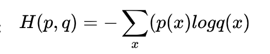
- Pytorch中CrossEntropyLoss()函数的主要是将softmax-log-NLLLoss合并到一块得到的结果。
1、Softmax后的数值都在0~1之间,所以ln之后值域是负无穷到0。
2、然后将Softmax之后的结果取log,将乘法改成加法减少计算量,同时保障函数的单调性 。
3、NLLLoss的结果就是把上面的输出与Label对应的那个值拿出来(下面例子中就是:将log_output\logsoftmax_output中与y_target对应的值拿出来),去掉负号,再求均值。
#set Loss function and optimizer
optimizer = optim.Adam(params = model.parameters(),lr=0.002)
# optimizer = optim.SGD(model.parameters(), lr=0.001, momentum=0.9)
criterion = nn.CrossEntropyLoss()

#check GPU
import tensorflow as tf
tf.test.gpu_device_name()
训练:
由于无法使用GPU训练所以训练速度很慢,只能使用25个epochs试验一下
#training
epochs = 25

for epoch in range(epochs):
    epoch_loss = 0
    epoch_accuracy = 0

    for data, label in train_loader:
        data = data.to(device)
        label = label.to(device)

        output = model(data)
        loss = criterion(output, label)

        optimizer.zero_grad()
        loss.backward()
        optimizer.step()

        acc = ((output.argmax(dim=1) == label).float().mean())
        epoch_accuracy += acc/len(train_loader)
        epoch_loss += loss/len(train_loader)

    print('Epoch : {}, train accuracy : {}, train loss : {}'.format(epoch+1, epoch_accuracy,epoch_loss))

    with torch.no_grad():
        epoch_val_accuracy=0
        epoch_val_loss =0
        for data, label in val_loader:
            data = data.to(device)
            label = label.to(device)

            val_output = model(data)
            val_loss = criterion(val_output,label)


            acc = ((val_output.argmax(dim=1) == label).float().mean())
            epoch_val_accuracy += acc/ len(val_loader)
            epoch_val_loss += val_loss/ len(val_loader)

        print('Epoch : {}, val_accuracy : {}, val_loss : {}'.format(epoch+1, epoch_val_accuracy,epoch_val_loss))
Tensorflow:
使用Adam优化器,损失函数为Tensorflow库的sparse_categorical_crossentropy
- 在 tf.keras 中,有两个交叉熵相关的损失函数 tf.keras.losses.categorical_crossentropy 和 tf.keras.losses.sparse_categorical_crossentropy 。其中 sparse 的含义是,真实的标签值 y_true 可以直接传入 int 类型的标签类别,即sparse时 y 不需要one-hot,而 categorical 需要。

#opt = Adam(lr=0.001)
#model.compile(optimizer = opt, loss = 'sparse_categorical_crossentropy', metrics = ['accuracy'])
#return model
#training the model
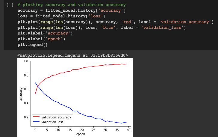
fitted_model = model.fit_generator(training_data,
                        steps_per_epoch = 200,
                        epochs = 40,
                        validation_data = testing_data,
                        validation_steps = 200)

若有收获,就点个赞吧
0 人点赞


